


Equilibrium Binding of Transcription Factors
If you know TF concentrations, binding site affinities, and cooperativities, can you predict probabilities for each configuration?
# imports
import os, sys
import string
import json
from collections import defaultdict
import itertools
from random import choice, random
import pickle
import requests
from xml.etree import ElementTree
import numpy as np
import pandas as pd
from scipy.stats import bernoulli, norm, lognorm, expon as exponential
from scipy.stats import rv_discrete, rv_continuous
from scipy.stats import hypergeom
from scipy import interpolate
import matplotlib
import matplotlib.pyplot as plt
import matplotlib as mpl
from matplotlib.text import TextPath
from matplotlib.font_manager import FontProperties
from matplotlib.collections import PolyCollection
from matplotlib.patches import Rectangle, Polygon, PathPatch
from matplotlib.colors import colorConverter, TABLEAU_COLORS, LinearSegmentedColormap
import matplotlib.cm as cm
from mpl_toolkits.mplot3d import axes3d
from mpl_toolkits.mplot3d import Axes3D
from matplotlib.ticker import MaxNLocator
# colorConverter.to_rgba('mediumseagreen', alpha=.5)
import matplotlib_inline.backend_inline
matplotlib_inline.backend_inline.set_matplotlib_formats('svg')
%config InlineBackend.figure_format = 'retina'
%matplotlib inline
plt.rcParams['figure.figsize'] = [12, 5]
plt.rcParams['figure.dpi'] = 140
plt.rcParams['agg.path.chunksize'] = 10000
plt.rcParams['animation.html'] = 'jshtml'
plt.rcParams['hatch.linewidth'] = 0.3
from IPython.display import display, HTML
from matplotlib_venn import venn2, venn3
import plotly.graph_objects as go
import seaborn as sns
# import seaborn.apionly as sns
sns.set_style("white")
import MOODS.tools
from dna_features_viewer import GraphicFeature, GraphicRecord
import pyBigWig
ln = np.log
exp = np.exp
# distribution plotting utilities
def is_discrete(dist):
if hasattr(dist, 'dist'):
return isinstance(dist.dist, rv_discrete)
else: return isinstance(dist, rv_discrete)
def is_continuous(dist):
if hasattr(dist, 'dist'):
return isinstance(dist.dist, rv_continuous)
else: return isinstance(dist, rv_continuous)
def plot_distrib(distrib, title=None):
fig, ax = plt.subplots(1, 1)
if is_continuous(distrib):
x = np.linspace(distrib.ppf(0.001),
distrib.ppf(0.999), 1000)
ax.plot(x, distrib.pdf(x), 'k-', lw=0.4)
elif is_discrete(distrib):
x = np.arange(distrib.ppf(0.01),
distrib.ppf(0.99))
ax.plot(x, distrib.pmf(x), 'bo', ms=2, lw=0.4)
r = distrib.rvs(size=1000)
ax.hist(r, density=True, histtype='stepfilled', alpha=0.2, bins=200)
if title: ax.set_title(title)
fig_style_2(ax)
return ax
def fig_style_2(ax):
for side in ["right","top","left"]: ax.spines[side].set_visible(False)
ax.get_yaxis().set_visible(False)
# functions for plotting DNA
base_colors = {'A': 'Lime', 'G': 'Gold', 'C': 'Blue', 'T':'Crimson'}
def print_bases(dna): return HTML(''.join([f'<span style="color:{base_colors[base]};font-size:1.5rem;font-weight:bold;font-family:monospace">{base}</span>' for base in dna]))
def print_dna(dna): return HTML(''.join([f'<span style="color:{base_colors[base]};font-size:1rem;font-family:monospace">{base}</span>' for base in dna]))
complement = {'A':'T', 'T':'A', 'C':'G', 'G':'C', 'a':'t', 't':'a', 'c':'g', 'g':'c'}
def reverse_complement(dna):
list_repr = [complement[base] for base in dna[::-1]]
if type(dna) == list: return list_repr
else: return ''.join(list_repr)
def reverse_complement_pwm(pwm, base_index='ACGT'):
return pwm[::-1, [base_index.index(complement[base]) for base in base_index]]
# gene name namespace_mapping utility
import mygene
def namespace_mapping(names, map_from=['symbol', 'alias'], map_to='symbol', species='human'):
names = pd.Series(names)
print(f"passed {len(names)} symbols")
names_stripped = names.str.strip()
if any(names_stripped != names):
print(f"{sum(names.str.strip() != names)} names contained whitespace. Stripping...")
names_stripped_unique = names_stripped.unique()
if len(names_stripped_unique) != len(names_stripped):
print(f"{len(names_stripped) - len(names_stripped_unique)} duplicates. {len(names_stripped_unique)} uniques.")
print()
mg = mygene.MyGeneInfo()
out, dup, missing = mg.querymany(names_stripped_unique.tolist(), scopes=map_from, fields=[map_to], species=species, as_dataframe=True, returnall=True).values()
out = out.reset_index().rename(columns={'query':'input'}).sort_values(['input', '_score'], ascending=[True, False]).drop_duplicates(subset='input', keep='first')
same = out[out.input == out.symbol]
updates = out[(out.input != out.symbol) & (out.notfound.isna() if 'notfound' in out else True)].set_index('input')['symbol']
print(f"\nunchanged: {len(same)}; updates: {len(updates)}; missing: {len(missing)}")
names_updated = updates.reindex(names_stripped.values)
names_updated = names_updated.fillna(names_updated.index.to_series()).values
return updates, missing, names_updated
# define read_shell() to read dataframe from shell output
import os, sys
import subprocess
import shlex
import io
def read_shell(command, shell=False, **kwargs):
proc = subprocess.Popen(command, shell=shell,stdout=subprocess.PIPE, stderr=subprocess.PIPE)
stdout, stderr = proc.communicate()
if proc.returncode == 0:
with io.StringIO(stdout.decode()) as buffer:
return pd.read_csv(buffer, **kwargs)
else:
message = ("Shell command returned non-zero exit status: {0}\n\n"
"Command was:\n{1}\n\n"
"Standard error was:\n{2}")
raise IOError(message.format(proc.returncode, command, stderr.decode()))
There exist two mathematical formalisms to describe the probabilities of molecular configurations at equilibrium: thermodynamics and kinetics. In the kinetics formalism, the system transits between configurational states according to rate parameters contained in differential equations, which can describe not just the system's equilibrium but also its trajectory towards it, or the kinetics of non-equilibrium systems. In the thermodynamics/statistical mechanics formalism, we posit that a system will occupy configurations with lower energy, and use the Boltzmann distribution to estimate the proportion of time the system spends in each state, at equilibrium. The thermodynamics formalism is limited to describing equilibrium state probabilities, but it does so with fewer parameters.
We'll derive an expression for the probability of a single TFBS' occupancy with both formalisms, but proceed with the thermodynamic description for more elaborate configurations. It will become clear why that is preferable.
Kinetics
Most derivations of the probability of single TFBS occupancy at equilibrium employ a kinetics formalism, so we'll walk through that first, and then explore the analog in the thermodynamics description. In the kinetics description, the parameters are rates.
$$ \mathrm{TF} + \mathrm{TFBS} \underset{\koff}{\overset{\kon}{\rightleftarrows}} \mathrm{TF\colon TFBS} $$
The natural rates are the rate of TF binding $\kon$ and unbinding $\koff$. Equilibrium is reached when binding and unbinding are balanced:
$$\frac{d[\mathrm{TF\colon TFBS}]}{dt} = k_{\mathrm{on}}[\mathrm{TF}][\mathrm{TFBS}] - k_{\mathrm{off}}[\mathrm{TF\colon TFBS}] = 0 \text{ at equilibrium}$$ $$k_{\mathrm{on}}[\mathrm{TF}]_{\mathrm{eq}}[\mathrm{TFBS}]_{\mathrm{eq}} = k_{\mathrm{off}}[\mathrm{TF\colon TFBS}]_{\mathrm{eq}}$$ $$\text{(dropping eq subscript) }[\mathrm{TF\colon TFBS}] = \frac{k_{\mathrm{on}}[\mathrm{TF}][\mathrm{TFBS}]}{k_{\mathrm{off}}} = \frac{[\mathrm{TF}][\mathrm{TFBS}]}{k_{d}}$$
where $k_{d} = \frac{\koff}{\kon}$ is called the dissociation constant (or equilibrium constant). We'd like to determine the probability of finding the TFBS occupied, i.e. the fraction of time it spends in the bound state. That fraction is $\frac{[\mathrm{bound}]}{([\mathrm{unbound}] + [\mathrm{bound}])} = \frac{[\mathrm{TF\colon TFBS}]}{([\mathrm{TFBS}] + [\mathrm{TF\colon TFBS}])}$. Define the denominator as $[\mathrm{TFBS}]_{0} = [\mathrm{TFBS}] + [\mathrm{TF\colon TFBS}]$ so that $[\mathrm{TFBS}] = [\mathrm{TFBS}]_{0} - [\mathrm{TF\colon TFBS}]$ and substitute:
$$[\mathrm{TF\colon TFBS}] = \frac{[\mathrm{TF}]([\mathrm{TFBS}]_{0} - [\mathrm{TF\colon TFBS}])}{k_{d}}$$ $$[\mathrm{TF\colon TFBS}](k_d + [\mathrm{TF}]) = [\mathrm{TF}][\mathrm{TFBS}]_{0}$$ $$\frac{[\mathrm{TF\colon TFBS}]}{[\mathrm{TFBS}]_{0}} = \frac{[\mathrm{TF}]}{k_d + [\mathrm{TF}]}$$
Thermodynamics
In the thermodynamics description, the parameters are Gibbs free energies $\Delta G$. Let's follow the derivation from Physical Biology of the Cell (pp. 242) and consider the number microstates underlying each of the of bound and unbound macrostates, and their energies.
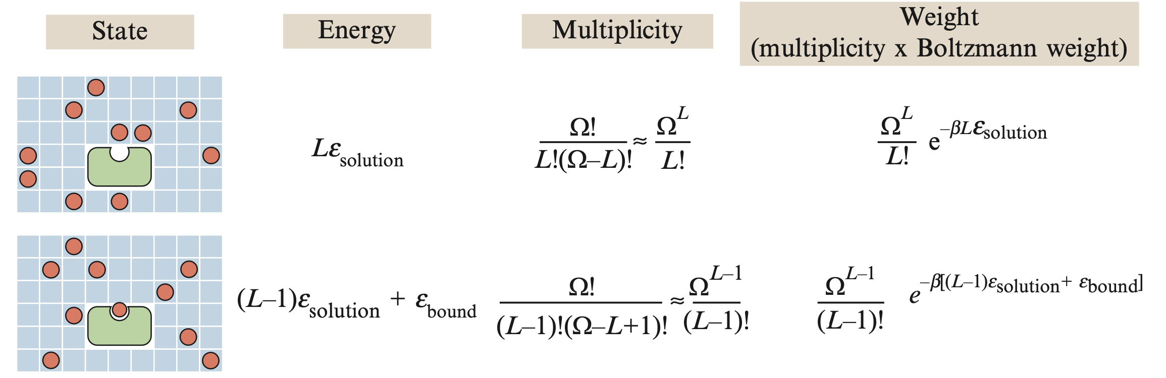
In order to count microstates, we imagine distributing $L$ TF molecules across a space-filling lattice with $\Omega$ sites. The energy of a TF in solution is $\varepsilon_{\mathrm{solution}}$ and the energy of a bound TF is $\varepsilon_{\mathrm{bound}}$. $\beta$ is the constant $1/k_b T$ where $k_b$ is Boltzmann's constant and $T$ is the temperature.
| State | Energy | Multiplicity | Weight |
 |
$A \cdot A_s$ | $\frac{\Omega!}{(\Omega - A)!A!} \approx \frac{\Omega^{A}}{A!}$ | $\frac{\Omega^{A}}{A!} \cdot e^{-\beta \left[ A \cdot A_s \right]}$ |
 |
$(A - 1) A_s + A_b$ | $\frac{\Omega!}{(\Omega - (A - 1))!(A-1)!B!} \approx \frac{\Omega^{A-1}}{(A-1)!}$ | $\frac{\Omega^{A-1}}{(A-1)!} \cdot e^{-\beta \left[ (A - 1) A_s + A_b \right]}$ |
In our case, the number of microstates in the unbound macrostate is $\frac{\Omega !}{L!(\Omega -L)!}\approx \frac{\Omega^L}{L!}$ and they each have energy $L \cdot \varepsilon_s$. The number of microstates in the bound macrostate is $\frac{\Omega !}{(L-1)!(\Omega -(L+1))}\approx \frac{\Omega^{(L-1)}}{(L-1)!}$ and they each have energy $(L-1) \varepsilon_s + \varepsilon_b$.
The Boltzmann distribution describes the probability of a microstate as a function of its energy: $p(E_i) = e^{-\beta E_i}/Z$ where $Z$ is the "partition function" or simply $\sum_i e^{-\beta E_i}$ the sum of the weights of the microstates, which normalizes the distribution. In our case:
$$Z(L,\Omega)=\left(\colorbox{LightCyan}{$ \frac{\Omega^L}{L!} e^{-\beta L \varepsilon_s}$}\right) + \left(\colorbox{Seashell}{$\frac{\Omega^{(L-1)}}{(L-1)!} e^{-\beta [(L-1) \varepsilon_s + \varepsilon_b]}$}\right)$$
With that expression in hand, we can express the probability of the bound macrostate, $p_b$:
$$p_b=\frac{ \colorbox{Seashell}{$\frac{\Omega^{(L-1)}}{(L-1)!} e^{-\beta [(L-1) \varepsilon_s + \varepsilon_b]}$}}{\colorbox{LightCyan}{$\frac{\Omega^L}{L!} e^{-\beta L \varepsilon_s}$} + \colorbox{Seashell}{$\frac{\Omega^{(L-1)}}{(L-1)!} e^{-\beta [(L-1) \varepsilon_s + \varepsilon_b]}$}} \cdot \color{DarkRed}\frac{\frac{\Omega^L}{L!}e^{\beta L \varepsilon_s}}{\frac{\Omega^L}{L!}e^{\beta L \varepsilon_s}} \color{black} = \frac{(L/\Omega)e^{- \beta \Delta \varepsilon}}{1+(L/\Omega)e^{- \beta \Delta \varepsilon}} $$
Where we have defined $\Delta \varepsilon = \varepsilon_b - \varepsilon_s$. $L/\Omega$ is really just a dimensionless TF concentration, which we'll hand-wave as being equivalent to $[\mathrm{TF}]$, which leaves us with an expression suspiciously similar to the one we derived from the kinetics formalism:
$$p_b = \frac{[\mathrm{TF}]e^{-\beta \Delta \varepsilon}}{1+[\mathrm{TF}]e^{-\beta \Delta \varepsilon}} \cdot \color{DarkRed}\frac{e^{\beta \Delta \varepsilon}}{e^{\beta \Delta \varepsilon}} \color{black} = \frac{[\mathrm{TF}]}{e^{\beta \Delta \varepsilon}+[\mathrm{TF}]}$$
From which we recapitulate an important correspondence between kinetics and thermodynamics at equilibrium: $ k_d = e^{\beta \Delta \varepsilon} = e^{\Delta \varepsilon / k_bT} $ more commonly written for different units as $k = e^{-\Delta G / RT}$.
The takeaway is that both the kinetics and thermodynamics formalisms produce an equivalent expression for the probabilities of each of the bound and unbound configurations, parameterized respectively by $k_d$ and $\Delta G$.
Sample Values
In order to compute probabilities like $p_b$, we need concrete TF concentrations $[\mathrm{TF}]$ and binding affinities (either $k_d$ or $\Delta G$). What are typical intranuclear TF concentrations and binding affinities?
Concentrations
A typical human cell line, K562s, have a cellular diameter of 17 microns. (BioNumbers)
def sphere_volume(d):
return 4/3*np.pi*(d/2)**3
K562_diameter_microns = 17
K562_volume_micron_cubed = sphere_volume(K562_diameter_microns)
print(f'K562 volume: {round(K562_volume_micron_cubed)} μm^3')
A typical expressed TF has a per-cell copy number range from $10^3$ - $10^6$. (BioNumbers)
copy_number_range = [1e3, 1e6]
N_A = 6.02214076e23
def copy_number_and_cubic_micron_volume_to_molar_concentration(copy_number, volume=K562_volume_micron_cubed):
return (copy_number / N_A) / (volume * (1e3 / 1e18)) # 1000 Liters / m^3; 1e18 μm^3 / m^3
lower_end_molar = copy_number_and_cubic_micron_volume_to_molar_concentration(copy_number_range[0], K562_volume_micron_cubed)
upper_end_molar = copy_number_and_cubic_micron_volume_to_molar_concentration(copy_number_range[1], K562_volume_micron_cubed)
lower_end_nanomolar = lower_end_molar / 1e-9
upper_end_nanomolar = upper_end_molar / 1e-9
print('If TF copy numbers range from 1,000-1,000,000, then TF concentrations range from', str(round(lower_end_nanomolar))+'nM', 'to', str(round(upper_end_nanomolar))+'nM')
We might also like a distribution over this range. Let's posit a lognormal, where $10^3$ and $10^6$ are the 3σ from the mean, which is $10^{4.5}$. Then $\sigma = 10^{0.5}$
# define a distribution over TF copy numbers
# Note: the lognormal is defined with base e, so we need to take some natural logs on our base 10 expression.
TF_copy_number_distrib = lognorm(scale=10**4.5, s=np.log(10**0.5))
ax = plot_distrib(TF_copy_number_distrib, title='Hypothetical expressed TF copy number distribution')
ax.set_xlim(left=0, right=5e5)
ax.set_xlabel('TF protein copy number / cell')
ax.get_xaxis().set_major_formatter(matplotlib.ticker.FuncFormatter(lambda x, p: format(int(x), ',')))
def TF_nanomolar_concentrations_sample(TFs):
return dict(zip(TFs, (copy_number_and_cubic_micron_volume_to_molar_concentration(TF_copy_number_distrib.rvs(len(TFs)))*1e9).astype(int)))

Affinities
What are typical TF ΔG's of binding? How about the $\koff$ rates and half lives?
- We can use the prior knowledge that dissociation constants should be in the nanomolar regime (BioNumbers).
- We can use the relation that $\Delta G = -k_b T \cdot \ln(k_d)$ (Plugging in 310°K (human body temp) and the Boltzmann constant $k_b$ in kcal/Mol)
- We use the approximation that $\kon$ is ~$10^5 / $ Molar $ \times $ sec (Wittrup)
T = 310
k_b = 3.297623483e-24 * 1e-3 ## cal/K * kcal/cal
kbT = k_b*T*N_A
kbT ## in 1/Mol -- an unusual format
k_on = 1e5
def nanomolar_kd_from_kcal_ΔG(ΔG): return exp(-ΔG/kbT) * 1e9
def kcal_ΔG_from_nanomolar_kd(K_d): return -kbT*ln(K_d*1e-9)
def k_off_from_nanomolar_kd(k_d): return (k_d*1e-9) * k_on
def half_life_from_kd(k_d): return ln(2) / ((k_d*1e-9) * k_on)
# compute statistics from kds
nanomolar_kds = pd.Series([1, 10, 100, 1000])
affinity_grid = pd.DataFrame()
affinity_grid['$k_d$'] = nanomolar_kds
affinity_grid['$\Delta G$'] = nanomolar_kds.apply(kcal_ΔG_from_nanomolar_kd)
affinity_grid['$\kon$'] = '1e5 / (M * s)'
affinity_grid['$\koff$'] = nanomolar_kds.apply(k_off_from_nanomolar_kd)
affinity_grid['$t_{1/2}$'] = pd.to_timedelta(nanomolar_kds.apply(half_life_from_kd), unit='s')
affinity_grid = affinity_grid.set_index('$k_d$')
affinity_grid
We learn that an order of magnitude residence time difference results from just 1.4 extra kcal/Mol, and that TF half lives range from about 5s to about 2h. Let's once again posit a distribution of affinities to sample from (defined on $k_d$):
# define a distribution over TF Kd's / ΔG's
TF_affinity_min = 6 ## define exponential distribution in log10 space
TF_affinity_spread = 0.5
TF_affinity_distrib = exponential(loc=TF_affinity_min, scale=TF_affinity_spread)
ax = plot_distrib(TF_affinity_distrib, title="Hypothetical TF $K_d$ distribution")
ax.set_xlim(left=5.9)
ax.set_xlabel('$k_d$')
plt.xticks([6,7,8,9], ['1000μm', '100nm', '10nm', '1nm'])
def TF_Kd_sample(n=1): return 10**(-TF_affinity_distrib.rvs(n))
def TF_ΔG_sample(n=1): return kcal_ΔG_from_nanomolar_kd(10**(-TF_affinity_distrib.rvs(n)+9))

With those concrete TF concentrations and dissociation constants, we can finally plot our function $p_b = \frac{[\mathrm{TF}]}{e^{\beta \Delta \varepsilon}+[\mathrm{TF}]}$.
@np.vectorize
def fraction_bound(TF, ΔG):
'''TF in nanomolar'''
return TF / (TF + nanomolar_kd_from_kcal_ΔG(ΔG))
# plot fraction bound as a function of concentration and binding energy
TF_concentration_array = np.logspace(1, 5)
ΔG_array = np.logspace(*np.log10([8, 13]))
TF_concs_matrix, ΔG_matrix = np.meshgrid(TF_concentration_array, ΔG_array)
z_data = pd.DataFrame(fraction_bound(TF_concs_matrix, ΔG_matrix), index=ΔG_array, columns=TF_concentration_array).rename_axis('ΔG').T.rename_axis('[TF]')
fig = go.Figure(data=[go.Surface(x=TF_concentration_array.astype(int).astype(str), y=ΔG_array.round(1).astype(str), z=z_data.values)])
fig.update_layout(
title='',
autosize=False,
width=700,
margin=dict(r=20, l=10, b=10, t=10),
scene = dict(
xaxis_title='[TF]',
yaxis_title='ΔG',
zaxis_title='Pb'),
scene_camera = dict(eye=dict(x=-1, y=-1.8, z=1.25)))
fig.update_traces(showscale=False)
# config = dict({'scrollZoom': False})
# fig.show(config = config)
# display(fig)
HTML(fig.to_html(include_plotlyjs='cdn', include_mathjax=False))
(Note that both $[\mathrm{TF}]$ and $k_d$ are plotted in log space, but $p_b$ is linear.)
As before, the statistical mechanics formalism entails enumerating the configurations, their multiplicities, and their energies. We'll call the TFs A and B. We'll denote their counts as $A$ and $B$. The energy of a TF in solution will once more be $A_s$ and bound to its cognate TFBS $A_b$. The energy of cooperativity will be $C_{AB}$.
| State | Energy | Multiplicity | Weight |
|
$A \cdot A_s + B \cdot B_s$ | $\frac{\Omega!}{(\Omega - A - B)!A!B!} \approx \frac{\Omega^{A+B}}{A!B!}$ | $\frac{\Omega^{A+B}}{A!B!} \cdot e^{-\beta \left[ A \cdot A_s + B \cdot B_s \right]}$ |
|
$(A - 1) A_s + A_b + B \cdot B_s$ | $\frac{\Omega!}{(\Omega - (A - 1) - B)!(A-1)!B!} \approx \frac{\Omega^{A+B-1}}{(A-1)!B!}$ | $\frac{\Omega^{A+B-1}}{(A-1)!B!} \cdot e^{-\beta \left[ (A - 1) A_s + A_b + B \cdot B_s \right]}$ |
 |
$A \cdot A_s + (B - 1) B_s + B_b$ | $\frac{\Omega!}{(\Omega - A - (B - 1))!A!(B-1)!} \approx \frac{\Omega^{A+B-1}}{A!(B-1)!}$ | $\frac{\Omega^{A+B-1}}{A!(B-1)!} \cdot e^{-\beta \left[ A \cdot A_s + (B - 1) B_s + B_b \right]}$ |
 |
$(A - 1) A_s + A_b + (B - 1) B_s + B_b + C_{AB}$ | $\frac{\Omega!}{(\Omega - (A - 1) - (B-1))!(A-1)!(B-1)!} \approx \frac{\Omega^{A+B-2}}{(A-1)!(B-1)!}$ | $\frac{\Omega^{A+B-2}}{(A-1)!(B-1)!} \cdot e^{-\beta \left[ (A - 1) A_s + A_b + (B - 1) B_s + B_b + C_{AB} \right]}$ |
The partition function is the sum of the weights:
$$ Z = \frac{\Omega^{A+B}}{A!B!} \cdot e^{-\beta \left[ A \cdot A_s + B \cdot B_s \right]} + \frac{\Omega^{A+B-1}}{(A-1)!B!} \cdot e^{-\beta \left[ (A - 1) A_s + A_b + B \cdot B_s \right]} + \frac{\Omega^{A+B-1}}{A!(B-1)!} \cdot e^{-\beta \left[ A \cdot A_s + (B - 1) B_s + B_b \right]} + \frac{\Omega^{A+B-2}}{(A-1)!(B-1)!} \cdot e^{-\beta \left[ (A - 1) A_s + A_b + (B - 1) B_s + B_b + C_{AB} \right]}$$Which we can greatly simplify by multiplying the entire expression by the reciprocal of the "base state" weight, $\color{DarkRed}\frac{A!B!}{\Omega^{A+B}} \cdot e^{\beta \left[ A \cdot A_s + B \cdot B_s \right]}$, normalizing that weight to 1:
$$ Z = 1 + \frac{A}{\Omega} \cdot e^{-\beta \left[ A_b-A_s \right]} + \frac{B}{\Omega} \cdot e^{-\beta \left[ B_b-B_s \right]} + \frac{A \cdot B}{\Omega^2} \cdot e^{-\beta \left[ A_b-A_s+B_b-B_s+C_{AB} \right]}$$Taking the definition $[A] = A/\Omega$ and $\Delta G_A = A_b-A_s$ produces:
$$ Z = 1 + [A] e^{-\beta \left[ \Delta G_A \right]} + [B] e^{-\beta \left[ \Delta G_B \right]} + [A][B] e^{-\beta \left[ \Delta G_A+\Delta G_B+C_{AB} \right]}$$Then the probability of any state is just the weight of that state (scaled by the weight of the base state) divided by the partition function expression $Z$.
From the above, we notice the form of the expression for the weight of a configuration of N TFBSs:
$$ p_{\mathrm{config}} = \prod_{i \in \, \mathrm{bound \,TBFS}} \left( [\mathrm{TF}_{\mathrm{cognate}(i)}] \cdot e^{-\beta \left[ \Delta G_i + \sum_j c_{ij} \right]} \right) / Z$$
For numerical stability, we take the log of the unnormalized probability (that is, the weight) of configurations:
$$ \log(\tilde{p}_{\mathrm{config}}) = \sum_{i \in \, \mathrm{bound \,TBFS}} \left( \log([\mathrm{TF}_{\mathrm{cognate}(i)}]) - \beta \left[ \Delta G_i + \sum_j c_{ij} \right] \right) $$
# define log_P_config()
β = 1/kbT ## kbT was in in 1/Mol
def log_P_config(config, TF_conc, TFBSs, cooperativities):
logP = 0
for i, tfbs in TFBSs[config.astype(bool)].iterrows():
cooperativity_sum = 0
if i in cooperativities:
cooperativity_sum = sum([C_AB for tfbs_j, C_AB in cooperativities[i].items() if config[tfbs_j] == 1])
logP = sum([np.log(TF_conc[tfbs.TF]*1e-9) + β*(tfbs.dG + cooperativity_sum)]) ## the sign is flipped here, because our ΔG's of binding are positive above.
return logP
Incorporating competition into our thermodynamic model is slightly more subtle than cooperativity, because we can imagine two types of competition
- Two TFs which may both bind DNA at adjacent sites, causing a free energy penalty due to some unfavorable interaction.
- Two TFs with overlapping DNA binding sites, which cannot physically be bound at the same time.
In the former case, the expression for $p_\mathrm{config}$ we had written before suffices, with values of $C_{AB}$ having both signs to represent cooperativity and competition. Nominally, the latter case also fits this formalism if we allow $C_{AB}$ to reach $-\infty$, but that would cause us headaches in the implementation. Instead, the weights of all those configurations which are not physical attainable, due to "strict" competitive binding between TFs vying for overlapping binding sites, are merely omitted from the denominator $Z$.
In order to compute concrete probabilities of configurations, accounting for cooperativity and competition, we will need concrete energies. We'll take $C_{AB}$ to be distributed exponentially with a mean at 2.2kcal/Mol. (Forsén & Linse).
# define a distribution of cooperativities
cooperativity_mean_ΔG = 2.2
cooperativity_distrib = exponential(scale=cooperativity_mean_ΔG)
ax = plot_distrib(cooperativity_distrib, title="Hypothetical $C_{AB}$ distribution")
ax.set_xlim(left=-0.5,right=15)
ax.set_xlabel('$C_{AB}$ (kcal/mol)')
def C_AB_sample(n=1): return cooperativity_distrib.rvs(n)

# sample that distribution for cooperativities between binding sites
def sample_cooperativities(TFBSs):
cooperativities = defaultdict(lambda: dict())
for i, tfbs_i in TFBSs.iterrows():
for j, tfbs_j in TFBSs.iterrows():
if i < j:
if 7 <= abs(tfbs_i.start - tfbs_j.start) <= 10:
cooperativities[i][j] = cooperativities[j][i] = C_AB_sample()[0]
elif abs(tfbs_i.start - tfbs_j.start) < 7:
cooperativities[i][j] = cooperativities[j][i] = -C_AB_sample()[0]
return dict(cooperativities)
Let's check our derivation (and our implementation) of $p_\mathrm{config}$ by comparing it to our direct computation of $p_b$ from §1. Single TF.
# define create_environment()
len_TFBS=10
def create_environment(len_DNA=1000, num_TFs=10, num_TFBS=20, len_TFBS=10):
# TFBSs is a dataframe with columns 'TF_name', 'start', 'dG'
TFs = list(string.ascii_uppercase[:num_TFs]) ## TF names are just letters from the alphabet
TF_conc = TF_nanomolar_concentrations_sample(TFs)
TFBSs = pd.DataFrame([{'TF': choice(TFs), 'start': int(random()*(len_DNA-len_TFBS)), 'dG': TF_ΔG_sample()[0]} for _ in range(num_TFBS)]).sort_values(by='start').reset_index(drop=True)
cooperativities = sample_cooperativities(TFBSs)
return TFs, TF_conc, TFBSs, cooperativities
# define draw_config() for plotting
def draw_config(TFBSs, TF_conc, cooperativities, config=None, len_DNA=1000):
if config is None: config = [0]*len(TFBSs)
TF_colors = dict(zip(list(TF_conc.keys()), list(TABLEAU_COLORS.values())))
plt.rcParams['figure.figsize'] = [12, 0.5+np.sqrt(len(TFs))]
fig, axs = plt.subplots(ncols=2, sharey=True, gridspec_kw={'width_ratios': [4, 1]})
genome_track_ax = draw_genome_track(axs[0], config, TFBSs, cooperativities, TF_colors, len_DNA=len_DNA)
conc_plot_ax = draw_concentration_plot(axs[1], TF_conc, TF_colors)
return genome_track_ax, conc_plot_ax
def draw_concentration_plot(conc_plot_ax, TF_conc, TF_colors):
conc_plot_ax.barh(range(len(TF_conc.keys())), TF_conc.values(), align='edge', color=list(TF_colors.values()), alpha=0.9)
for p in conc_plot_ax.patches:
conc_plot_ax.annotate(str(p.get_width())+'nm', (p.get_width() + 10*(p.get_width()>0), p.get_y() * 1.02), fontsize='x-small')
conc_plot_ax.axes.get_yaxis().set_visible(False)
conc_plot_ax.axes.get_xaxis().set_visible(False)
conc_plot_ax.set_frame_on(False)
return conc_plot_ax
def draw_genome_track(genome_track_ax, config, TFBSs, cooperativities, TF_colors, len_DNA=1000):
genome_track_ax.set(ylabel='TFs', ylim=[-1, len(TF_colors.keys())+1], yticks=range(len(TFs)), yticklabels=TFs, xlabel='Genome', xlim=[0, len_DNA])
for i, tfbs in TFBSs.iterrows():
tfbs_scale = np.clip(0.01*np.exp(tfbs.dG-7), 0, 1)
genome_track_ax.add_patch(Rectangle((tfbs.start, TFs.index(tfbs.TF)), len_TFBS, 0.8, fc=TF_colors[tfbs.TF], alpha=tfbs_scale))
genome_track_ax.add_patch(Rectangle((tfbs.start, TFs.index(tfbs.TF)), len_TFBS, 0.1*tfbs_scale, fc=TF_colors[tfbs.TF], alpha=1))
genome_track_ax.annotate(str(int(tfbs.dG))+'kcal/Mol', (tfbs.start, TFs.index(tfbs.TF)-0.3), fontsize='xx-small')
genome_track_ax.add_patch(Polygon([[tfbs.start+2, TFs.index(tfbs.TF)], [tfbs.start+5,TFs.index(tfbs.TF)+0.8],[tfbs.start+8, TFs.index(tfbs.TF)]], fc=TF_colors[tfbs.TF], alpha=config[i]))
cm = matplotlib.cm.ScalarMappable(norm=matplotlib.colors.Normalize(vmin=-3, vmax=3), cmap=matplotlib.cm.PiYG)
for i, rest in cooperativities.items():
for j, C_AB in rest.items():
tfbs_i = TFBSs.iloc[i]
tfbs_j = TFBSs.iloc[j]
xa = tfbs_i.start+(len_TFBS/2)
xb = tfbs_j.start+(len_TFBS/2)
ya = TFs.index(tfbs_i.TF)
yb = TFs.index(tfbs_j.TF)
genome_track_ax.plot([xa, (xa+xb)/2, xb], [ya+0.9, max(ya, yb)+1.2, yb+0.9], color=cm.to_rgba(C_AB))
genome_track_ax.grid(axis='y', lw=0.1)
genome_track_ax.set_frame_on(False)
return genome_track_ax
def enumerate_configs(TFBSs): return list(map(np.array, itertools.product([0,1], repeat=len(TFBSs))))
def p_configs(TFBSs, TF_conc, cooperativities):
configs = enumerate_configs(TFBSs)
weights = []
for config in configs:
weights.append(np.exp(log_P_config(config, TFBSs=TFBSs, TF_conc=TF_conc, cooperativities=cooperativities)))
return list(zip(configs, np.array(weights) / sum(weights)))
TFs, TF_conc, TFBSs, cooperativities = create_environment(len_DNA=100, num_TFs=1, num_TFBS=1)
print('p_bound (prev method): \t', fraction_bound(TF_conc['A'], TFBSs.iloc[0].dG))
print('p_config (new method): \t', p_configs(TFBSs=TFBSs, TF_conc=TF_conc, cooperativities={}))
genome_track_ax, conc_plot_ax = draw_config(TFBSs=TFBSs, TF_conc=TF_conc, cooperativities=cooperativities, len_DNA=100)
plt.tight_layout()

With that sanity check, let's now consider the scenario of two transcription factors with cooperative binding, and compute the probabilities of each of the 4 configurations:
# Create cooperative environment
len_DNA = 100
TFs = ['A', 'B']
TF_conc = TF_nanomolar_concentrations_sample(TFs)
TFBSs = pd.DataFrame([{'TF': 'A', 'start': 10, 'dG': TF_ΔG_sample()[0]}, {'TF': 'B', 'start': 20, 'dG': TF_ΔG_sample()[0]}])
cooperativities = {0: {1: 2}, 1: {0: 2}}
TF_colors = dict(zip(list(TF_conc.keys()), list(TABLEAU_COLORS.values())))
plt.rcParams['figure.figsize'] = [12, 2*(0.8+int(np.sqrt(len(TFs))))]
fig, axs = plt.subplots(nrows=2, ncols=2)
for ax, (config, p) in zip([ax for row in axs for ax in row], p_configs(TFBSs=TFBSs, TF_conc=TF_conc, cooperativities=cooperativities)):
draw_genome_track(ax, config, TFBSs, cooperativities, TF_colors, len_DNA=50)
ax.set(ylabel='', xlabel='')
ax.set_title('$p_\mathrm{config}$: '+str(round(p*100,3))+'%', y=1.0, pad=-28, loc='left', fontsize=10)

Low-Affinity binding
In reality, transcription factors' binding sites are not so discretely present or absent: transcription factors may bind anywhere along the DNA polymer, with an affinity dependent on the interaction surface provided by the sequence of nucleotides at each locus. There are a variety of approaches to model the sequence-to-affinity function for each TF. The simplest is to consider each nucleotide independently, and list the preferences for each nucleotide at each sequential position in a matrix. This type of "mono-nucleotide position weight matrix" (PWM) model is commonly used, and frequently represented by a "sequence logo" plot.
tfdb2 = pd.read_json('../../AChroMap/data/processed/TF.2022.json').fillna(value=np.nan) ## prefer nan to None
cisbp_pwms = pd.read_pickle('../../tfdb/data/processed/CISBP_2_PWMs.pickle')
humanTFs_pwms = pd.read_pickle('../../tfdb/data/processed/HumanTFs_PWMs.pickle')
jaspar2022_pwms = pd.read_pickle('../../tfdb/data/processed/jaspar2022_PWMs.pickle')
probound_pwms = pd.read_json('../../AChroMap/data/processed/TF_ProBound.json', orient='records').T # we only get probound as delta G scores, not as PWMs
SPI1_pwms = tfdb2.loc[(tfdb2.Name == 'SPI1')]
SPI1_cisbp_pwms = cisbp_pwms.loc[SPI1_pwms.CISBP_2_strict.iat[0]]
SPI1_humanTFs_pwms = humanTFs_pwms.reindex(SPI1_pwms.HumanTFs.iat[0]).dropna()
SPI1_jaspar2022_pwms = jaspar2022_pwms.loc[SPI1_pwms.JASPAR_2022.iat[0]]
SPI1_probound_pwms = probound_pwms.loc[SPI1_pwms.ProBound.iat[0]].pwm
# plot PWMs
def hide_axes_and_spines(ax, hide_x_axis=True, hide_y_axis=True, spines_to_hide=['right','top','left','bottom']):
for side in spines_to_hide:
ax.spines[side].set_visible(False)
if hide_x_axis:
ax.get_xaxis().set_visible(False)
if hide_y_axis:
ax.get_yaxis().set_visible(False)
fp = FontProperties(family="Arial", weight="bold")
globscale = 1.35
LETTERS = { "T" : TextPath((-0.305, 0), "T", size=1, prop=fp),
"G" : TextPath((-0.384, 0), "G", size=1, prop=fp),
"A" : TextPath((-0.35, 0), "A", size=1, prop=fp),
"C" : TextPath((-0.366, 0), "C", size=1, prop=fp) }
def letterAt(letter, x, y, yscale=1, ax=None):
text = LETTERS[letter]
t = mpl.transforms.Affine2D().scale(1*globscale, yscale*globscale) + \
mpl.transforms.Affine2D().translate(x,y) + ax.transData
p = PathPatch(text, lw=0, fc=base_colors[letter], transform=t, alpha=1-0.8*(y<0))
if ax != None:
ax.add_artist(p)
return p
def plot_pwm(pwm, ax=None, base_index='ACGT', figsize=(4,2), xtick_offset=0):
if ax is None: fig, ax = plt.subplots(figsize=figsize)
max_y = 0
min_y = 0
for i, row in enumerate(pwm):
x = xtick_offset+i
pos_y = 0
neg_y = -0.1
for score, base in sorted(zip(row, base_index)):
if score > 0:
letterAt(base, x,pos_y, score, ax=ax)
pos_y += score
if score < 0:
neg_y += score
letterAt(base, x,neg_y, abs(score), ax=ax)
max_y = max(max_y, pos_y)
min_y = min(min_y, neg_y)
ax.set(xticks=range(-1,len(pwm)+xtick_offset), xlim=(-1, len(pwm)+xtick_offset), ylim=(min_y, max_y))
if min_y < -0.1:
ax.set_ylabel('ΔΔG/RT', weight='bold')
hide_axes_and_spines(ax, hide_y_axis=False)
else:
hide_axes_and_spines(ax)
plt.tight_layout()
return ax
for (name, SPI1_pwm), offset in zip(SPI1_cisbp_pwms.items(), (0,0,2,0,0,0)):
ax = plot_pwm(SPI1_pwm, figsize=((len(SPI1_pwm)+offset+1)*0.25,1), xtick_offset=offset)
ax.set_title(name, loc='left')


This representation of this matrix visualizes the proportion of occurrences of a base at a particular position in aligned SPI1 binding sites. Since they look similar, we may be tempted to average them to have a single model of PU.1 binding, however it is considered unwise to do so, as TFs are believed to have multiple binding "modes" which refers explicitly to modes in the distribution of sequence-binding affinities.
These PWM models can be fit from a variety of experiments measuring PU.1 binding. In this case, we're looking at models fit from High-Throughput SELEX data, but other models for PU.1 binding generated from other types of experiments are catalogued at its entry in the HumanTFs database.
If we assume a TF's PWM catalogues its relative binding preferences to every possible sequence of individual bases, we can use that PWM to evaluate the relative probabilities of TF binding to new sequences. We'll define the PWM "score" as the (log) ratio of the probability of the sequence with the PWM against random chance. The probability of a sequence under the PWM is $\prod \mathrm{PWM}[i][\mathrm{dna}[i]]$. The probability of the sequence under a background model is $\prod \mathrm{bg}(\mathrm{dna}[i])$ where $\mathrm{bg}$ describes the frequency of each base in the genome (not quite 1/4 in the human genome). We take the logarithm of the ratio of these two probabilities to produce the log-likelihood ratio, which we call our "score":
$$\mathrm{score}(\mathrm{PWM}, j) = \log(\frac{\prod \mathrm{PWM}[i][\mathrm{dna}[j+i]]}{\prod \mathrm{bg}(\mathrm{dna}[j+i])}) = \sum \log(\frac{ \mathrm{PWM}[i][\mathrm{dna}[j+i]]}{\mathrm{bg}(\mathrm{dna}[j+i])}) $$
A positive $\mathrm{score}(\mathrm{PWM}, j)$ indicates the subsequence starting at position $j$ is likelier under the PWM model than a random sequence from the human genome, and a negative score indicates the subsequence is more likely to be random. Let's visualize a PU.1 scoring matrix:
bg = [0.2955, 0.2045, 0.2045, 0.2955]
pseudocount = 0.0001
def log_odds_pwm(pwm):
return np.log((pwm+pseudocount)/bg)
pwm = SPI1_cisbp_pwms.iloc[1]
pwm_name = SPI1_cisbp_pwms.index[0]
ax = plot_pwm(log_odds_pwm(pwm), figsize=(4,4))
_ = ax.set_ylabel('score', weight='bold')

cisbp_score_pwms = cisbp_pwms.apply(log_odds_pwm)
humanTFs_score_pwms = humanTFs_pwms.apply(log_odds_pwm)
jaspar2022_score_pwms = jaspar2022_pwms.apply(log_odds_pwm)
SPI1_cisbp_score_pwms = cisbp_score_pwms.loc[SPI1_pwms.CISBP_2_strict.iat[0]]
SPI1_humanTFs_score_pwms = humanTFs_score_pwms.reindex(SPI1_pwms.HumanTFs.iat[0]).dropna()
SPI1_jaspar2022_score_pwms = jaspar2022_score_pwms.loc[SPI1_pwms.JASPAR_2022.iat[0]]
Our strategy will be to score genomic regions for TF binding, searching for high PWM scores starting at every offset $j$ in the supplied DNA sequence. Let's remind ourselves here that in order to find the full set of motif matches in a supplied DNA sequence, we either need to scan the reference genome and its reverse complement, or scan the positive strand with both the forward and reverse-complement PWMs. We opt for the latter approach, and therefore augment our PWM set with reverse-complement PWMs:
plot_pwm(pwm, figsize=(4,1)).set_title('Forward: '+pwm_name, loc='left')
plot_pwm(reverse_complement_pwm(pwm), figsize=(4,1)).set_title('Reverse: '+pwm_name, loc='left')
None


Since we now have sequence-dependent transcription factor binding models, we will select a sequence which harbors known binding sites for select transcription factors, and see whether the models predict binding of those transcription factors.
As a specific sequence, let's use the SPI1 promoter.
def get_reference_transcript(gene_name):
hg38_reference_annotation = pd.read_csv('../../AChroMap/data/processed/GRCh38_V29.csv')
reference_transcript = hg38_reference_annotation[(hg38_reference_annotation.gene_name == gene_name) & (hg38_reference_annotation.canonicity == 0)]
chrom = reference_transcript.chr.iat[0]
strand = reference_transcript.strand.iat[0]
tss = (reference_transcript.txStart if all(reference_transcript.strand == 1) else reference_transcript.txEnd).iat[0]
return chrom, strand, tss
gene_name = 'SPI1'
chrom, strand, tss = get_reference_transcript(gene_name)
start = tss-400
stop = tss+400
def get_hg38_bases_local(chrom, start, stop):
seqkit_command = f'seqkit subseq /Users/alex/Documents/AChroMap/data/raw/genome/hg38_fa/{chrom}.fa --region {start}:{stop}'
dna = subprocess.run(shlex.split(seqkit_command), stdout=subprocess.PIPE).stdout.decode('utf-8').split('\n',1)[1].replace('\n','')
return dna
SPI1_promoter_dna_sequence = get_hg38_bases_local(chrom, start, stop)
print(SPI1_promoter_dna_sequence)
SPI1 promotes its own transcription, by binding to its own promoter. We can scan the SPI1 promoter for significant SPI1 PWM scores to locate the binding site.
base_index = {'a':0,'c':1,'g':2,'t':3,'A':0,'C':1,'G':2,'T':3}
def scan_sequence(pwm, dna):
scores = []
for i in range(len(dna)):
score = 0
for j, row in enumerate(pwm):
if i+j < len(dna):
score += row[base_index[dna[i+j]]]
scores.append(score)
return np.array(scores)
SPI1_PWM_scores = pd.DataFrame(SPI1_cisbp_score_pwms.apply(scan_sequence, args=(SPI1_promoter_dna_sequence,)).values.tolist(), index=SPI1_cisbp_score_pwms.index).T
SPI1_PWM_scores.index += start
positive_SPI1_PWM_scores = pd.DataFrame(np.where(SPI1_PWM_scores > 0, SPI1_PWM_scores, np.nan), index=SPI1_PWM_scores.index, columns=SPI1_PWM_scores.columns)
def genomic_xticks(ax, chrom=None):
xlims = ax.get_xlim()
xtick_vals = ax.get_xticks()
ax.set_xticks(xtick_vals)
ax.set_xticklabels(['{:.0f}'.format(x) for x in xtick_vals])
ax.set_xlim(xlims)
if chrom: ax.set_xlabel(chrom)
ax = SPI1_PWM_scores.plot(lw=0.1, xlim=(SPI1_PWM_scores.index.min(),SPI1_PWM_scores.index.max()), legend=False)
ax = positive_SPI1_PWM_scores.plot(style=".", ax=ax)
ax.set_ylabel('score')
genomic_xticks(ax)
def plot_tss(ax, tss, strand, axvline=False):
arrow_direction = 8 if strand == -1 else 9
ax.plot(tss, 1, lw=0, markersize=10, c='deepskyblue', marker=arrow_direction)
ax.text(tss+1,0,gene_name)
if axvline: ax.axvline(tss, c='deepskyblue', lw=0.5)
plot_tss(ax, tss, strand)
Now we'd like to score every PWM against every offset in the entire reference human genome. In order to accomplish that, we'll use MOODS, which implements a faster scanning algorithm in C++. We'll use this script to score the human reference genome with our PWMs.
Once we have scanned a sequence of genomic DNA, scoring the PWM at every offset, we need to establish which of those scores is "significant" enough that we would predict the existence of a transcription factor binding site at that position in the genome. We can imagine two approaches to distinguish "significant" motif matches for each PWM. Thresholding on a particular score corresponds to predicting the TF is bound to sites which are $e^{\mathrm{score}}$ more likely under the PWM than random. A score cutoff of 6.91 is 1000x more likely under the PWM than random, for every PWM.
Contrarily, if you wanted to choose the 0.1% top scores for each PWM, each PWM would have a unique score cutoff, as each cutoff would depend on the distribution of scores specified by the PWM. At first this may seem surprising, so we'll explore it empirically for two PWMs:
pwm_names = ['M07944_2.00','M03355_2.00']
pwms = cisbp_pwms.loc[pwm_names]
score_pwms = cisbp_score_pwms.loc[pwm_names]
for name, pwm in pwms.items(): plot_pwm(pwm, figsize=(4,1)).set_title(name, loc='left')


def sample_scores_from_pwm(pwm, sample_size=int(1e6)):
scores = np.zeros(sample_size)
for i in range(len(pwm)):
scores += np.random.choice(pwm[i], sample_size, p=bg)
return pd.Series(scores)
score_samples = score_pwms.apply(sample_scores_from_pwm).T
ax = score_samples.plot.hist(bins=100, alpha=0.5)
ax.set(xlabel='score')
fig_style_2(ax)

Clearly we can see these two PWMs define different score distributions for random sequences. Let's see what probabilities the highest scores correspond to for each of these PWMs, using MOODS' score cutoff method:
def score_thresholds(score_pwm):
min_significance, max_significance = -2, -15
significance_range = min_significance - max_significance
pvals = np.logspace(min_significance, max_significance, significance_range*2+1)
score_thresholds = [MOODS.tools.threshold_from_p(score_pwm.T.tolist(), bg, p) for p in pvals]
return pd.Series(score_thresholds, index=pvals)
score_quantiles = score_pwms.apply(score_thresholds).T.rename_axis('p').reset_index()
fig, ax = plt.subplots()
cols = score_quantiles.columns[1:]
for col in cols:
score_quantiles.plot(x=col, y='p', logy=True, legend=False, ax=ax)
ax.set(ylabel='p_value', xlabel='score')
ax.grid(True, ls=':')
for side in ["right","top"]: ax.spines[side].set_visible(False)
ax.legend(cols)
ax.axhline(1e-3, c='red')
ax.text(0,2e-3, 'p=0.001')
ax.plot(score_quantiles.iloc[2][['M07944_2.00','M03355_2.00']],(1e-3, 1e-3), marker='o', lw=0, c='red')
None

For each motif, we can compute which score corresponds to each p-value cutoff, and then estimate p-values for scores of motif matches discovered during scanning using an interpolation. We'll use a generic spline as an interpolation function.
# cisbp_score_quantiles.to_csv('../data/equilibrium_TFs/cisbp_score_quantiles.csv', index=False)
cisbp_score_quantiles = pd.read_csv('../notebook_data/equilibrium_TFs/cisbp_score_quantiles.csv')
def create_score_to_pval_interpolant(motif_name):
quantiles = cisbp_score_quantiles[[motif_name, 'p']]
quantiles = quantiles[quantiles[motif_name] >= quantiles[motif_name].cummax()].drop_duplicates(subset=[motif_name], keep='first') # guarantee strict monotonic increasing
score_to_pval_interpolation = interpolate.InterpolatedUnivariateSpline(quantiles[motif_name], quantiles['p'], ext=3)
return score_to_pval_interpolation
# create_score_to_pval_interpolant(motif_name)
# tfbs.loc[tfbs.name == motif_name, 'p'] = tfbs.loc[tfbs.name == motif_name, 'score'].apply(score_to_pval_interpolation)
Unfortunately, the PWM formalism we have introduced misses the biophysical interpretation we have carried throughout our analysis thus far. We can coax a biophysical interpretation from these PWMs as follows (following the approach from Foat, Morozov, Bussemaker, 2006):
If we consider the nucleotides independently, then the ratio of equilibrium binding to a given nucleotide $j$ versus the highest-affinity nucleotide $\mathrm{best}$ at each position is related to the difference in energies of binding:
$$ \frac{[TF:N_j]}{[TF:N_{best}]} = \frac{K_{a_j}}{K_{a_{best}}} = \exp \{\Delta G_j - \Delta G_{best} \} $$
With this expression, we can compute the energy of binding of a TF to a sequence relative to that TF's energy of binding to its best sequence of nucleotides. However, we need to know an absolute energy of binding to anchor this relative measure.
cisbp_energy_pwms = cisbp_pwms.apply(make_energy_pwm)
humanTFs_energy_pwms = humanTFs_pwms.apply(make_energy_pwm)
jaspar2022_energy_pwms = jaspar2022_pwms.apply(make_energy_pwm)
We can visualize this "energy PWM" as well. Visualizing energies of particular bases relative to SPI1's best sequence does not produce a visual representation that's easy to reason about:
SPI1_cisbp_energy_pwms = cisbp_energy_pwms.loc[SPI1_cisbp_pwms.index]
SPI1_cisbp_energy_pwm = SPI1_cisbp_energy_pwms[0]
ax = plot_pwm(SPI1_cisbp_energy_pwm)

We can rescale this matrix to the average sequence:
ax = plot_pwm(SPI1_cisbp_energy_pwm - np.expand_dims(SPI1_cisbp_energy_pwm.mean(axis=1), axis=1))

However, the ideal rescaling of this PWM would indicate whether each nucleotide contributes positively or negatively towards the energy of binding. After all, SPI1 likely doesn't bind the "average" sequence -- which is to say it's off rate is higher than it's on rate.
We chose SPI1 / PU.1 as our prototype in part because its absolute binding energies to various sequences have been measured, allowing us to anchor our relative energies PWM model. Pham et al measured PU.1 binding to a variety of high-affinity sequences by microscale thermophoresis and recorded a $k_d$ of 156nm for the best one.
SPI1_best_nanomolar_kd = 156
SPI1_best_ΔG = kcal_ΔG_from_nanomolar_kd(SPI1_best_nanomolar_kd)
SPI1_best_ΔG
However, the question remains of how to allocate those ~9.6 kcal/mol across the 14 bases of the SPI1 motif. The naive option is to uniformly spread the binding energy across the bases (9.6/14). Instead, we'll distribute it proportionally to the variance at each position to capture the intuition that the flanking nucleotides contribute less.
# define make_abs_pwm()
def make_abs_pwm(pwm, ΔG_of_best_sequence):
'''each base is allocated the absolute value of the variation at that position'''
if str(pwm) == 'nan': return np.nan
energy_range = abs(np.min(pwm, axis=1))
energy_fractional_allocation = energy_range/energy_range.sum()
energy_per_base = ΔG_of_best_sequence * energy_fractional_allocation
abs_pwm = pwm + np.expand_dims(energy_per_base, axis=1)
return abs_pwm
SPI1_cisbp_energy_pwm_scaled = make_abs_pwm(SPI1_cisbp_energy_pwm, SPI1_best_ΔG)
ax = plot_pwm(SPI1_cisbp_energy_pwm_scaled)

At last we have a visual representation of of a mono-nucleotide sequence preference model which captures our intuitions about the energetics of TF binding.
For a restricted set of TFs with high-quality HT-SELEX data, Rube et al produced relative energy PWMs with higher accuracy in the low-affinity regime. SPI1 is among that privileged set, so we'll take a look at that PWM for comparison.
SPI1_probound_pwms_scaled = SPI1_probound_pwms.apply(lambda pwm: make_abs_pwm(pwm, SPI1_best_ΔG))
ax = plot_pwm(SPI1_probound_pwms_scaled.iloc[2])

To what extent do these PWM models predict real transcription factor binding? In order to evaluate these models, we would like to compare their predictions with ground truth measurements of transcription factor occupancy.
- TF occupancy can be estimated with ChIP. Has been estimated in K562 (and HepG2)
Limitations:
- We only have PWMs for 1000 TFs,
- We only have ChIP for 600 TFs
What's the intersection?
all_chip_able_targets = pd.read_csv('/Users/alex/Documents/AChroMap/data/raw/ENCODE/k562_chip/metadata.cleaned.tsv', sep='\t').Target
pwm_cols = ['CISBP_2_strict','CISBP_2_intermediate','CISBP_2_tolerant','HumanTFs','JASPAR_2022','ProBound']
TF_coverage = {pwm_db: tfdb2[tfdb2.set_index('Name')[pwm_db].notnull().values].Name for pwm_db in pwm_cols}
fig, axs = plt.subplots(2, len(pwm_cols)//2)
for pwm_db, ax in zip(pwm_cols, axs.flatten()):
colors = ['dodgerblue', 'seagreen', 'lightsteelblue']
venn_obj = venn3((set(TF_coverage[pwm_db]), set(all_chip_able_targets), set(tfdb2.Name)),
(f'{pwm_db} ({len(set(TF_coverage[pwm_db]))})', f'ChIP in K562 ({len(set(all_chip_able_targets))})', f'DNA-binding TF ({len(set(tfdb2.Name))})'),
colors, alpha=0.6, ax=ax)
for text in venn_obj.set_labels: text.set_fontsize(8)
for text in [x for x in venn_obj.subset_labels if x]: text.set_fontsize(6)
venn_obj.set_labels[0].set_fontweight(700)
venn_obj.get_patch_by_id('111').set_edgecolor('green')

TFs_to_evaluate = set(all_chip_able_targets) & set(TF_coverage['CISBP_2_strict'])
pd.Series(list(TFs_to_evaluate)).to_csv('../notebook_data/TFs_to_evaluate.csv', index=False, header=False)
- Justify only looking inside ATAC peaks / OCRs.
explain motivation: want to look in all ATAC regions for PWMs and chip signal in k562s
narrowpeak_cols = ['chrom','chromStart','chromEnd','name','score','strand','signalValue','pValue','qValue','summit']
ATAC_peaks_files = ['/Users/alex/Documents/AChroMap/data/raw/ENCODE/k562_atac/downloads/ENCFF333TAT.bed',
'/Users/alex/Documents/AChroMap/data/raw/ENCODE/k562_atac/downloads/ENCFF558BLC.bed']
ATAC_signal_files = ['/Users/alex/Documents/AChroMap/data/raw/ENCODE/k562_atac/downloads/ENCFF357GNC.bigWig',
'/Users/alex/Documents/AChroMap/data/raw/ENCODE/k562_atac/downloads/ENCFF600FDO.bigWig']
def filter_overlapping_peaks_for_max_signalValue(filepath, fraction_either=0.8):
narrowpeaks_unfiltered = pd.read_csv(f'{filepath}', sep='\t', na_values=['NAN'], header=None, names=narrowpeak_cols)
bedops_command = f"bedops -u {filepath} | cut -f1-4,7 | bedmap --fraction-either {fraction_either} --max-element - | sort-bed --unique - > {filepath}.tmp"
os.system(bedops_command)
narrowPeaks_filtered_peak_names = pd.read_csv(f'{filepath}.tmp', sep='\t', na_values=['NAN'], header=None, names=narrowpeak_cols[:5]).name
os.remove(f'{filepath}.tmp')
return narrowpeaks_unfiltered[narrowpeaks_unfiltered.name.isin(narrowPeaks_filtered_peak_names)]
K562_ATAC_peaks_1_filtered = filter_overlapping_peaks_for_max_signalValue(ATAC_peaks_files[0])
K562_ATAC_peaks_2_filtered = filter_overlapping_peaks_for_max_signalValue(ATAC_peaks_files[1])
K562_ATAC_peaks_1_filtered['signalValue_percentile'] = K562_ATAC_peaks_1_filtered.signalValue.rank(pct=True)
K562_ATAC_peaks_2_filtered['signalValue_percentile'] = K562_ATAC_peaks_2_filtered.signalValue.rank(pct=True)
def get_overlapping_peaks(peaks_bed, chrom, start, stop):
intervals = pd.IntervalIndex.from_arrays(peaks_bed.chromStart, peaks_bed.chromEnd)
return peaks_bed[(peaks_bed.chrom == chrom) & intervals.overlaps(pd.Interval(start, stop))]
atac_peak_at_SPI1_promoter_1 = get_overlapping_peaks(K562_ATAC_peaks_1_filtered, chrom, start, stop)
atac_peak_at_SPI1_promoter_2 = get_overlapping_peaks(K562_ATAC_peaks_2_filtered, chrom, start, stop)
# plot Open Chromatin Regions overlapping SPI1 promoter from two separate K562 bulk ATAC-seq experiments.
earliest_start = min(start, atac_peak_at_SPI1_promoter_1.chromStart.iat[0], atac_peak_at_SPI1_promoter_2.chromStart.iat[0])
latest_end = max(stop, atac_peak_at_SPI1_promoter_1.chromEnd.iat[0], atac_peak_at_SPI1_promoter_2.chromEnd.iat[0])
plot_dna_length = (latest_end - earliest_start)*1.1
offset = earliest_start - plot_dna_length*0.05
features = [
GraphicFeature(start=start, end=stop, color="#ffd700", label="±400bp 'promoter' around tss"),
GraphicFeature(start=tss-30, end=tss, strand=-1, color="#ffcccc", label="tss"),
GraphicFeature(start=atac_peak_at_SPI1_promoter_1.chromStart.iat[0], end=atac_peak_at_SPI1_promoter_1.chromEnd.iat[0], color="#cffccc", label="peak called in ATAC dataset 1"),
GraphicFeature(start=atac_peak_at_SPI1_promoter_2.chromStart.iat[0], end=atac_peak_at_SPI1_promoter_2.chromEnd.iat[0], color="#ccccff", label="peak called in ATAC dataset 2")
]
record = GraphicRecord(features=features, sequence_length=latest_end*1.2)
cropped_record = record.crop((offset, offset+plot_dna_length))
ax, rest = cropped_record.plot(figure_width=10)
plt.setp(ax.get_xticklabels(), fontsize=7)
None

def get_bigwig_values(url, chrom, start, stop):
with pyBigWig.open(url) as bw:
values = bw.values(chrom, start, stop)
return values
ATAC_bigwig_1 = get_bigwig_values(ATAC_signal_files[0], chrom, earliest_start, latest_end)
ATAC_bigwig_2 = get_bigwig_values(ATAC_signal_files[1], chrom, earliest_start, latest_end)
ATAC_bigwig = pd.DataFrame([ATAC_bigwig_1, ATAC_bigwig_2], columns=range(earliest_start, latest_end), index=['ATAC_1', 'ATAC_2']).T
ax = ATAC_bigwig.plot.line()
plot_tss(ax, tss, strand)
genomic_xticks(ax)

from this we conclude that the first set of ATAC peaks is a richer dataset, and proceed with those
ATAC_OCRs_to_evaluate_PWMs_in = K562_ATAC_peaks_1_filtered[K562_ATAC_peaks_1_filtered.score == 1000]
ATAC_OCRs_to_evaluate_PWMs_in.to_csv('../notebook_data/equilibrium_TFs/K562_ATAC_peaks_filtered.bed', sep='\t', index=False)
motif_cluster_and_gene = pd.read_csv('/Users/alex/Documents/AChroMap/data/raw/Vierstra_supp/motif_cluster_and_gene.csv', index_col=0)
motif_clusters_to_TFs = pd.read_csv('/Users/alex/Documents/AChroMap/data/raw/Vierstra_supp/motif_clusters_to_TFs.csv', index_col=0)
motif_clusters_to_TFs = motif_clusters_to_TFs.set_index('Name')['gene'].str.split(';')
DGF_footprint_index = pd.read_csv('/Users/alex/Documents/AChroMap/data/raw/Vierstra_supp/consensus_index_matrix_full_hg38.index.csv', index_col=0, header=None).index
DGF_samples_index = pd.read_csv('/Users/alex/Documents/AChroMap/data/raw/Vierstra_supp/consensus_index_matrix_full_hg38.columns.csv', index_col=0, header=None).index
K562_DGF_samples = DGF_samples_index[DGF_samples_index.str.startswith('K562')].tolist()
def get_k562_DGF(chrom, start, end):
dgf_path = '/Users/alex/Documents/AChroMap/data/raw/Vierstra_supp/consensus_footprints_and_collapsed_motifs_hg38.bed.gz'
tabix_coords = chrom+':'+str(start)+'-'+str(end)
cols = ['contig','start','stop','identifier','mean_signal','num_samples','num_fps','width','summit_pos','core_start','core_end','motif_clusters']
tabix_command = f'tabix {dgf_path} {tabix_coords}'
footprints_contained_in_region = read_shell(shlex.split(tabix_command), sep='\t', header=None, names=cols, dtype={'index_id': str})
footprints_contained_in_region['TFs'] = footprints_contained_in_region.motif_clusters.str.split(';').apply(lambda l: [motif_clusters_to_TFs[motif_cluster] for motif_cluster in l] if (type(l) == list) else [])
first_dgf_index = DGF_footprint_index.get_loc(footprints_contained_in_region.identifier.iloc[0])
last_dgf_index = DGF_footprint_index.get_loc(footprints_contained_in_region.identifier.iloc[-1])+1
footprint_posterior = pd.read_hdf('/Users/alex/Documents/AChroMap/data/raw/Vierstra_supp/consensus_index_matrix_full_hg38.hdf', key='consensus_index_matrix_full_hg38',
start=first_dgf_index, stop=last_dgf_index, columns=K562_DGF_samples)
footprint_binary = pd.read_hdf('/Users/alex/Documents/AChroMap/data/raw/Vierstra_supp/consensus_index_matrix_binary_hg38.hdf', key='consensus_index_matrix_full_hg38',
start=first_dgf_index, stop=last_dgf_index, columns=K562_DGF_samples)
k562_dgf = footprints_contained_in_region.merge(footprint_posterior, how='left', left_on='identifier', right_index=True)
k562_dgf = k562_dgf.merge(footprint_binary, how='left', left_on='identifier', right_index=True, suffixes=['_posterior','_binary'])
return k562_dgf
k562_dgf = get_k562_DGF(chrom, start, stop)
k562_dgf.plot.scatter(x='K562-DS15363_posterior', y='K562-DS16924_posterior', figsize=(4,4), logx=True, logy=True)
ENCODE_RNA_metadata = pd.read_csv('../../AChroMap/data/raw/ENCODE/rna/metadata.tsv', sep='\t')
ENCODE_RNA_metadata_cleaned = pd.read_csv('../../AChroMap/data/raw/ENCODE/rna/metadata.clean.typed.csv')
ENCODE_polyA_metadata = pd.read_csv('../../AChroMap/data/raw/ENCODE/polyA/metadata.tsv', sep='\t')
ENCODE_polyA_metadata_cleaned = pd.read_csv('../../AChroMap/data/raw/ENCODE/polyA/metadata.clean.typed.csv')
rna_counts = pd.read_csv('../../AChroMap/data/raw/ENCODE/rna/RSEM_gene/RSEM_gene.counts_matrix.wellexpressed_deseq.csv', index_col=0)
polyA_counts = pd.read_csv('../../AChroMap/data/raw/ENCODE/polyA/RSEM_gene/RSEM_gene.counts_matrix.wellexpressed_deseq.csv', index_col=0)
K562_reference_polyA = pd.read_csv('/Users/alex/Desktop/ENCFF472HFI.tsv', sep='\t')
K562_reference_polyA = K562_reference_polyA[K562_reference_polyA.gene_id.str.startswith('ENSG')]
K562_reference_polyA['gene_id'] = K562_reference_polyA.gene_id.str.split('.').str[0]
K562_reference_polyA = K562_reference_polyA.set_index('gene_id')
K562_RNA_metadata = ENCODE_RNA_metadata[ENCODE_RNA_metadata['Biosample term name'] == 'K562']
K562_RNA_metadata_cleaned = ENCODE_RNA_metadata_cleaned[ENCODE_RNA_metadata_cleaned['Biosample term name'] == 'K562']
K562_polyA_metadata = ENCODE_polyA_metadata[ENCODE_polyA_metadata['Biosample term name'] == 'K562']
K562_polyA_metadata_cleaned = ENCODE_polyA_metadata_cleaned[ENCODE_polyA_metadata_cleaned['Biosample term name'] == 'K562']
K562_RNA_metadata_cleaned = K562_RNA_metadata_cleaned[K562_RNA_metadata_cleaned.type == 'RSEM_gene']
K562_polyA_metadata_cleaned = K562_polyA_metadata_cleaned[K562_polyA_metadata_cleaned.type == 'RSEM_gene']
K562_RNA_metadata = K562_RNA_metadata[K562_RNA_metadata['File accession'].isin(K562_RNA_metadata_cleaned.file)]
K562_polyA_metadata = K562_polyA_metadata[K562_polyA_metadata['File accession'].isin(K562_polyA_metadata_cleaned.file)]
K562_RNA_metadata = K562_RNA_metadata[K562_RNA_metadata['Audit WARNING'].isnull() & K562_RNA_metadata['Audit ERROR'].isnull() & K562_RNA_metadata['Audit NOT_COMPLIANT'].isnull()]
K562_polyA_metadata = K562_polyA_metadata[K562_polyA_metadata['Audit WARNING'].isnull() & K562_polyA_metadata['Audit ERROR'].isnull() & K562_polyA_metadata['Audit NOT_COMPLIANT'].isnull()]
K562_RNA_metadata_cleaned = K562_RNA_metadata_cleaned[K562_RNA_metadata_cleaned.file.isin(K562_RNA_metadata['File accession'])]
K562_polyA_metadata_cleaned = K562_polyA_metadata_cleaned[K562_polyA_metadata_cleaned.file.isin(K562_polyA_metadata['File accession'])]
K562_rna_counts = rna_counts.loc[rna_counts.index.str.startswith('ENSG'), rna_counts.columns.isin(K562_RNA_metadata['File accession'])]
K562_polyA_counts = polyA_counts.loc[polyA_counts.index.str.startswith('ENSG'), polyA_counts.columns.isin(K562_polyA_metadata['File accession'])]
K562_rna_counts.index = K562_rna_counts.index.str.split('.').str[0]
K562_polyA_counts.index = K562_polyA_counts.index.str.split('.').str[0]
best_polyA_files = K562_polyA_metadata_cleaned[K562_polyA_metadata_cleaned.experiment.isin(['ENCSR000AEP','ENCSR000AEQ'])].file.tolist()
best_rna_files = K562_RNA_metadata_cleaned[K562_RNA_metadata_cleaned.experiment.isin(['ENCSR792OIJ'])].file.tolist()
def series_to_distplot(s):
sns.kdeplot(data=s)
sns.rugplot(data=s, height=.1)
rna_counts_sum = K562_rna_counts.sum()
series_to_distplot(rna_counts_sum)
ax = plt.gca()
for x in rna_counts_sum[best_rna_files].values:
ax.axvline(x, c='r', lw=0.3)
plt.subplots()
polyA_counts_sum = K562_polyA_counts.sum()
series_to_distplot(polyA_counts_sum)
ax = plt.gca()
for x in polyA_counts_sum[best_polyA_files].values:
ax.axvline(x, c='r', lw=0.3)
mRNAs_per_cell = 1e5 # citation follows
RNAs_per_cell = 4e5 # this one is a guess
K562_polyA_TPC = K562_polyA_counts / K562_polyA_counts.sum() * mRNAs_per_cell
K562_rna_TPC = K562_rna_counts / K562_rna_counts.sum() * RNAs_per_cell
K562_RNA_TF_TPC = K562_rna_TPC[K562_rna_TPC.index.isin(tfdb2.ID)]
K562_polyA_TF_TPC = K562_polyA_TPC[K562_polyA_TPC.index.isin(tfdb2.ID)]
K562_polyA_TF_TPC.index = tfdb2.set_index('ID').reindex(K562_polyA_TF_TPC.index).Name.values
plt.rcParams['figure.figsize'] = [17, 5]
g = sns.stripplot(data=K562_polyA_TF_TPC.iloc[:100].T, alpha=0.4)
plt.xticks(rotation=-90)
g = sns.stripplot(data=K562_polyA_TF_TPC.iloc[:100][best_polyA_files].T, color='black', s=2, marker="D")
# also plot the median
None
K562_polyA_TF_TPC.to_csv('../notebook_data/equilibrium_TFs/K562_TF_RNA.csv')
RNA_to_protein_linear_scaling_factor = 9800
K562_TF_copy_number = K562_polyA_TF_TPC.replace(0, np.nan).median(axis=1).replace(np.nan, 0) * RNA_to_protein_linear_scaling_factor
plt.rcParams['figure.figsize'] = [12, 5]
K562_TF_copy_number.plot.hist(bins=100, logy=True)
K562_TF_nanomolar_conc = K562_TF_copy_number.apply(copy_number_and_cubic_micron_volume_to_molar_concentration, args=(K562_volume_micron_cubed,)) * 1e9
K562_TF_RNA_concise = pd.concat((tfdb2.set_index('Name').ID.reindex(K562_TF_copy_number.index),
K562_TF_copy_number.rename('TF_protein_copy_number_estimate'),
K562_TF_nanomolar_conc.rename('nanomolar_conc')), axis=1)
K562_TF_RNA_concise = K562_TF_RNA_concise.rename_axis('Name').reset_index().set_index('ID')
K562_TF_RNA_concise = K562_TF_RNA_concise.sort_values('TF_protein_copy_number_estimate', ascending=False).drop_duplicates(subset=['Name'])
K562_TF_RNA_concise.to_csv('../notebook_data/equilibrium_TFs/K562_TF_RNA_concise.csv')
We've just generated a list of OCRs we want to evaluate PWMs for, but let's start with our single example to determine how to evaluate PWMs vs ChIP.
# chrom, strand, tss = get_reference_transcript(gene_name)
# start = tss-400
# stop = tss+400
# K562_TF_RNA = pd.read_csv('../notebook_data/equilibrium_TFs/K562_TF_RNA.csv', index_col=0)
def get_K562_TF_ChIP_peaks(chrom, start, end):
k562_merged_ChIP_path = '/Users/alex/Documents/AChroMap/data/raw/ENCODE/k562_chip/K562_ChIP_merged.bed.gz'
tabix_coords = chrom+':'+str(start)+'-'+str(end)
tabix_command = f'tabix {k562_merged_ChIP_path} {tabix_coords}'
peaks_contained_in_region = read_shell(shlex.split(tabix_command), sep='\t', header=None, names=['chrom','chromStart','chromEnd','name','signalValue'])
return peaks_contained_in_region
K562_SPI1_TF_chip_peaks = get_K562_TF_ChIP_peaks(chrom, start, stop)
peaks_df = K562_SPI1_TF_chip_peaks[K562_SPI1_TF_chip_peaks.name.isin(TFs_to_evaluate)]
SPI1_promoter_TF_ChIP_signal = pd.read_csv('../notebook_data/equilibrium_TFs/SPI1_promoter_TF_ChIP_signal.csv', index_col=0)
SPI1_promoter_TF_ChIP_signal = SPI1_promoter_TF_ChIP_signal.clip(lower=1).replace(1, np.nan)
signal_df = SPI1_promoter_TF_ChIP_signal.loc[:, SPI1_promoter_TF_ChIP_signal.columns.str.split('_').str[0].isin(TFs_to_evaluate)]
signal_df = signal_df[signal_df.max(axis=0).sort_values(ascending=False).index.values]
SPI1_promoter_TF_ATAC_signal = pd.Series(get_bigwig_values(ATAC_signal_files[0], chrom, start, stop), index=range(start, stop), name='ATAC_signal')
SPI1_promoter_TF_ATAC_signal = SPI1_promoter_TF_ATAC_signal.clip(lower=1).replace(1, np.nan)
SPI1_key = f'{chrom}/{atac_peak_at_SPI1_promoter_1.chromStart.iat[0]}-{atac_peak_at_SPI1_promoter_1.chromEnd.iat[0]}'
SPI1_cisbp_tfbs = pd.read_hdf('../../AChroMap/scripts/cisbp2_vs_chip.hdf', SPI1_key)
SPI1_cisbp_tfbs = SPI1_cisbp_tfbs[(SPI1_cisbp_tfbs.start > start) & (SPI1_cisbp_tfbs.end < stop)]
SPI1_cisbp_tfbs['p'] = SPI1_cisbp_tfbs.p.clip(lower=1e-10)
SPI1_cisbp_tfbs['log10p'] = -np.log10(SPI1_cisbp_tfbs.p)
signal_df = SPI1_promoter_TF_ChIP_signal.loc[:, SPI1_promoter_TF_ChIP_signal.columns.str.split('_').str[0].isin(TFs_to_evaluate)]
TF_order = signal_df.max(axis=0).sort_values().index.str.split('_').str[0].drop_duplicates(keep='first')
column_order = pd.Series({col: (TF_order.get_loc(col.split('_')[0]), int(col.split('_')[1])) for col in signal_df.columns}).sort_values().index
signal_df = signal_df[column_order]
signal_df_20 = signal_df.iloc[:, -20:]
columns_to_TF = signal_df_20.columns.to_frame()[0].str.split('_').str[0].rename('TF').rename_axis('track').reset_index().reset_index().set_index('track')
TF_to_columns = columns_to_TF.reset_index().set_index('TF')
plotted_TFs = set(TF_to_columns.index)
genome_linspace = np.transpose(np.tile(signal_df_20.index.values, (len(signal_df_20.T), 1)))
print('genome_linspace:', genome_linspace.shape)
signal_heights = signal_df_20.values
print('signal_heights:\t', signal_heights.shape)
TF_y_index = np.linspace(0,len(signal_df_20.columns)-1,len(signal_df_20.columns))
print('TF_y_index: \t', TF_y_index.shape)
signal_verts = []
for y_i in range(len(TF_y_index)):
# zero at the beginning and the end to get a nice flat bottom on the polygons
xs = np.concatenate([[genome_linspace[0,y_i]], genome_linspace[:,y_i], [genome_linspace[-1,y_i]]])
ys = np.concatenate([[0],signal_heights[:,y_i],[0]])
signal_verts.append(list(zip(xs, ys)))
colors = LinearSegmentedColormap('colormap', cm.jet._segmentdata.copy(), 20)
colors = [colors(i) for i in range(20)]
peak_verts = []
peak_offsets = []
for col, d in columns_to_TF.iterrows():
for i, peak in peaks_df[peaks_df['name'] == d.TF].iterrows():
xs = [peak.chromStart, peak.chromStart, peak.chromEnd, peak.chromEnd]
ys = [0, peak.signalValue/20, peak.signalValue/20, 0]
peak_verts.append(list(zip(xs, ys)))
peak_offsets.append(d['index'])
tfbs_verts = []
tfbs_offsets = []
for col, d in columns_to_TF.iterrows():
for i, tfbs in SPI1_cisbp_tfbs[SPI1_cisbp_tfbs['TFs'] == d.TF].iterrows():
xs = [tfbs.start, tfbs.start, tfbs.end, tfbs.end]
ys = [0, tfbs.score/50, tfbs.score/50, 0]
tfbs_verts.append(list(zip(xs, ys)))
tfbs_offsets.append(d['index'])
plt.rcParams['figure.figsize'] = [10, len(signal_df.columns)]
fig = plt.figure()
ax = fig.add_subplot(111, projection='3d')
signal_poly = PolyCollection(signal_verts, facecolors=colors)
signal_poly.set_alpha(0.7)
ax.add_collection3d(signal_poly, zs=TF_y_index, zdir='y')
peak_poly = PolyCollection(peak_verts, edgecolors=(0,0,0,0.3), facecolors=(0,0,0,0))
# peak_poly.set_alpha(0.4)
ax.add_collection3d(peak_poly, zs=peak_offsets, zdir='y')
tfbs_poly = PolyCollection(tfbs_verts)
tfbs_poly.set_alpha(1)
ax.add_collection3d(tfbs_poly, zs=tfbs_offsets, zdir='y')
ax.set_xlim3d(genome_linspace.min(), genome_linspace.max())
ax.set_xlabel(chrom)
ax.set_ylim3d(TF_y_index.min(), TF_y_index.max())
ax.set_ylabel('TF')
ax.set_zlim3d(signal_heights.min(), signal_heights.max())
ax.set_zlabel('signal fold change over background')
xtick_vals = ax.get_xticks()
ax.set_xticks(xtick_vals)
ax.set_xticklabels(['{:.0f}'.format(x) for x in xtick_vals])
ax.set_yticks(TF_y_index)
ax.set_yticklabels(signal_df.columns)
ax.xaxis.pane.fill = False
ax.yaxis.pane.fill = False
ax.zaxis.pane.fill = False
ax.xaxis.pane.set_edgecolor('w')
ax.yaxis.pane.set_edgecolor('w')
ax.zaxis.pane.set_edgecolor('w')
ax.grid(False)
ax.get_proj = lambda: np.dot(Axes3D.get_proj(ax), np.diag([1.0, 1.5, 1.0, 1.0]))
plt.show()
import matplotlib.style as mplstyle
mplstyle.use('fast')
def style_ax(ax):
ax.spines['top'].set_visible(False)
ax.spines['right'].set_visible(False)
ax.spines['bottom'].set_visible(False)
ax.patch.set_alpha(0)
from matplotlib.ticker import Locator
class MinorSymLogLocator(Locator):
"""
Dynamically find minor tick positions based on the positions of
major ticks for a symlog scaling.
"""
def __init__(self, linthresh):
"""
Ticks will be placed between the major ticks.
The placement is linear for x between -linthresh and linthresh,
otherwise its logarithmically
"""
self.linthresh = linthresh
def __call__(self):
'Return the locations of the ticks'
majorlocs = self.axis.get_majorticklocs()
# iterate through minor locs
minorlocs = []
# handle the lowest part
for i in range(1, len(majorlocs)):
majorstep = majorlocs[i] - majorlocs[i-1]
if abs(majorlocs[i-1] + majorstep/2) < self.linthresh:
ndivs = 10
else:
ndivs = 9
minorstep = majorstep / ndivs
locs = np.arange(majorlocs[i-1], majorlocs[i], minorstep)[1:]
minorlocs.extend(locs)
return self.raise_if_exceeds(np.array(minorlocs))
def tick_values(self, vmin, vmax):
raise NotImplementedError('Cannot get tick locations for a '
'%s type.' % type(self))
def style_stripplot(ax):
ax.set_xscale('symlog', linthresh=2)
ax.get_xaxis().set_major_formatter(matplotlib.ticker.ScalarFormatter())
# ax.xaxis.grid(True, which='minor')
ax.set_xlim([0, 200])
ax.set_xticks([0, 1, 10, 100, 200])
ax.xaxis.set_minor_locator(MinorSymLogLocator(1e-1))
signal_df2 = signal_df[signal_df.max(axis=0).sort_values(ascending=False).index.values].iloc[:, :10]
K562_polyA_TF_TPC_medians = K562_polyA_TF_TPC.replace(0, np.nan).median(axis=1).fillna(0)
# I want a nucleosome binding energy track on this figure
# chip peaks could be triangles or some other shape -- especially if we had the summit
# are the summits always in the middle?
# show the motif on the screen somewhere?
# fully featured genomics feature track?
# plot the problem statement
# maybe I should be plotting the TF's p-values rather than scores? coloring by correlation or something?
# TFBS: 2 colors: below threshold and above threshold
plot_chip_peaks = True
plot_chip_signal = True
plot_atac_signal = True
plot_tfbs = True
plot_dgf = True
num_rows = 1+len(signal_df2.columns)
plt.rcParams['figure.figsize'] = [18, num_rows]
plt.rcParams['path.simplify_threshold'] = 1.0
TF_names = signal_df2.columns.str.split('_').str[0].unique()
fig, axs = plt.subplots(len(TF_names), 2, sharex='col', gridspec_kw={'width_ratios': [3, 1]})
left_axs = [row[0] for row in axs]
row_dict = dict(zip(TF_names, axs[:-1]))
if plot_atac_signal:
SPI1_promoter_TF_ATAC_signal.plot.line(ax=left_axs[-1], ylim=(0, SPI1_promoter_TF_ATAC_signal.max()), xlim=(start, stop), c='black', label='ATAC')
left_axs[-1].set_ylabel('ATAC', rotation=0)
plot_tss(left_axs[-1], tss, strand, axvline=True)
style_ax(left_axs[-1])
for i, (TF_name, row) in enumerate(row_dict.items()):
row[0].set_xlim([start, stop])
row[0].set_ylim([0, 30])
style_ax(row[0])
color = 'darkblue' if i%2 == 0 else 'royalblue'
for uid in signal_df2.loc[:, signal_df2.columns.str.split('_').str[0] == TF_name].columns:
line = row[0].plot(signal_df2.index.values, signal_df2[uid].values, label=uid, clip_on=False, color=color, lw=1)
# ax.legend(handles=line, loc='upper left', borderaxespad=0, frameon=False)
g1 = sns.stripplot(data=K562_polyA_TF_TPC.loc[TF_name].to_frame(), x=TF_name, orient='h', alpha=0.5, c='lightblue', ax=row[1])
g2 = sns.stripplot(data=K562_polyA_TF_TPC.loc[TF_name, best_polyA_files].to_frame(), x=TF_name, orient='h', color='red', ax=row[1])
g3 = sns.stripplot(data=K562_polyA_TF_TPC_medians.to_frame().loc[[TF_name]].T, x=TF_name, orient='h', color='black', marker='D', ax=row[1])
style_ax(row[1])
row[1].set_xlim(0, K562_polyA_TF_TPC.max().max())
row[1].set_ylabel(TF_name, rotation=0)
# row[1].set_xscale('symlog', linthresh=1)
# row[1].plot(K562_polyA_TF_TPC_medians.at[TF_name], TF_name, 'ko')
if i == 0:
row[1].spines['top'].set_visible(True)
style_stripplot(row[1])
if plot_chip_peaks:
for index, peak in peaks_df.iterrows():
if peak['name'] in row_dict.keys():
ax = row_dict[peak['name']][0]
ax.add_patch(Rectangle((peak.chromStart, 0), peak.chromEnd-peak.chromStart, 30, fc=(1,0,0,np.clip(0.0005*peak.signalValue, a_min=0, a_max=1)), ec=(1,0,0,0.1), zorder=-1, clip_on=False))
if plot_tfbs:
tfbs_cm = matplotlib.cm.ScalarMappable(norm=matplotlib.colors.Normalize(vmin=0, vmax=20), cmap=matplotlib.cm.OrRd)
for index, tfbs in SPI1_cisbp_tfbs.iterrows():
if tfbs['TFs'] in row_dict.keys():
ax = row_dict[tfbs['TFs']][0]
ax.add_patch(Rectangle((tfbs.start, 0), tfbs.end-tfbs.start, (tfbs.log10p-2)*4, fc=tfbs_cm.to_rgba(tfbs.log10p), ec=(0,0,0,0), zorder=10, clip_on=False))
# fc=(0,1,0,np.clip(0.01*tfbs.log10p, a_min=0, a_max=1)),
if plot_dgf:
last_ax = left_axs[-1]
for index, dgf in k562_dgf.iterrows():
alpha = 0.005*(dgf['K562-DS15363_posterior'] + dgf['K562-DS16924_posterior'])/2
_,top = fig.transFigure.inverted().transform(left_axs[0].transAxes.transform([0,1]))
_,bottom = fig.transFigure.inverted().transform(left_axs[-1].transAxes.transform([0,0]))
trans = matplotlib.transforms.blended_transform_factory(left_axs[0].transData, fig.transFigure)
fig.add_artist(Rectangle((dgf.core_start,bottom), dgf.core_end-dgf.core_start, top-bottom, transform=trans, fc=(0,0,1,alpha), ec=None, zorder=-10))
genomic_xticks(left_axs[-1], chrom=chrom)
axs[-1][1].axis('off')
axs[0][1].xaxis.set_tick_params(labeltop=True)
plt.savefig('/Users/alex/Desktop/SPI1_promoter_K562_TF_ChIP.png')
None
max_chip_peak_height = peaks_df.groupby('name')['signalValue'].max().rename('max_chip_peak_height')
max_chip_peak_height
def set_colors(df, x_col, y_col):
df['c'] = np.nan
df.loc[(df[y_col] > 0) & (df[x_col] > 0), 'c'] = 'g'
df.loc[(df[y_col] > 0) & (df[x_col] <= 0), 'c'] = 'm'
df.loc[(df[y_col] <= 0) & (df[x_col] > 0), 'c'] = 'r'
df.loc[(df[y_col] <= 0) & (df[x_col] <= 0), 'c'] = 'c'
return df
K562_TF_RNA = pd.read_csv('../../back_of_my_envelope/data/equilibrium_TFs/K562_TF_RNA.csv', index_col=0)
K562_TF_RNA = K562_TF_RNA.replace(0, np.nan).median(axis=1).replace(np.nan, 0).rename('TF_RNA')
K562_TF_RNA
def process_peak_tfbs_df(tfbs_df):
tfbs_df = tfbs_df[tfbs_df.TFs.isin(TFs_to_evaluate)]
tfbs_df.p.clip(lower=1e-10, upper=None, inplace=True)
tfbs_df['log10p'] = -np.log10(tfbs_df.p)
tfbs_df = tfbs_df.merge(max_chip_peak_height, how='left', left_on='TFs', right_index=True)
tfbs_df = tfbs_df.merge(K562_TF_RNA, how='left', left_on='TFs', right_index=True)
tfbs_df['score_x_RNA'] = ln(exp(tfbs_df['score']) * tfbs_df['TF_RNA'])
tfbs_df['log10p_x_RNA'] = tfbs_df['log10p'] * tfbs_df['TF_RNA']
return tfbs_df.reset_index(drop=True)
# distance to peak center
# dgf
tfbs_df = process_peak_tfbs_df(SPI1_cisbp_tfbs)
def lims(series, buffer=0.01):
spread = series.max() - series.min()
limits = (series.min() - spread*buffer, series.max() + spread*buffer)
return limits
def log_lims(series, log_buffer=1):
lower = np.log10(series[series > 0].min()) - log_buffer
upper = np.log10(series[series > 0].max()) + log_buffer
return (lower, upper)
def spearman_corr(df, tfbs_col, chip_col): return df.loc[:, [tfbs_col, chip_col]].corr(method='spearman').loc[tfbs_col, chip_col]
spearman_corr(tfbs_df, 'score', 'max_signal'), spearman_corr(tfbs_df, 'score_x_RNA', 'max_signal')
def plot_peak_scatter(df, mode='hist', x_col='score', y_col='max_signal', log=False, legend=False, ylim=(-0.1, 20)):
palette={'g':'g','m':'m','r':'r','c':'c'}
df = set_colors(df, x_col, y_col)
df['chip_signalBinary'] = (df[y_col] > 0).astype(int)
df['pwm_scoreBinary'] = (df[x_col] > 0).astype(int)
g = sns.JointGrid(data=df, x=x_col, y=y_col, xlim=lims(df[x_col]), ylim=ylim, hue='c', palette=palette)
g.plot_joint(sns.scatterplot, alpha=0.2, s=5, legend=legend)
if mode == 'hist':
sns.histplot(data=df, x=x_col, bins=100, ax=g.ax_marg_x, hue='chip_signalBinary', palette={0:'r', 1:'g'}, legend=False, log_scale=(False, True),element="step")
if log:
sns.histplot(data=df, y=y_col, bins=[0, 1]+np.logspace(1, 5).tolist(), ax=g.ax_marg_y, hue='pwm_scoreBinary', palette={0:'m', 1:'g'}, legend=False, log_scale=(True, False),element="step")
else:
sns.histplot(data=df, y=y_col, bins=200, ax=g.ax_marg_y, hue='pwm_scoreBinary', palette={0:'m', 1:'g'}, legend=False, log_scale=(True, False),element="step")
g.ax_marg_y.tick_params(labeltop=True)
g.ax_marg_y.grid(True, axis='x', ls=':')
g.ax_marg_x.tick_params(labelleft=True)
g.ax_marg_x.grid(True, axis='y', ls=':')
elif mode=='kde':
sns.kdeplot(data=df, x=x_col, ax=g.ax_marg_x, hue='chip_signalBinary', palette={0:'r', 1:'g'}, fill=True, alpha=0.1, legend=False)
sns.kdeplot(data=df, y=y_col, ax=g.ax_marg_y, hue='pwm_scoreBinary', palette={0:'m', 1:'g'}, fill=True, alpha=0.1, legend=False, log_scale=(False, True))
g.fig.set_figwidth(10)
g.fig.set_figheight(5)
corr = spearman_corr(df, x_col, y_col)
g.fig.suptitle(f'Spearman_correlation: {round(corr, 4)}')
if legend:
handles, labels = g.ax_joint.get_legend_handles_labels()
replacement = {'g':'Motif match and ChIP peak',
'm':'ChIP peak without motif match',
'r':'Motif match without ChIP peak',
'c':'Neither motif match nor ChIP Peak'}
labels = [replacement[x] for x in labels]
legend = g.ax_joint.legend(handles, labels, loc='upper left')
if log:
g.ax_joint.set_yscale('symlog', linthresh=min(0.1, df[df.max_signal > 0].max_signal.min()))
return g, corr
g = plot_peak_scatter(tfbs_df, x_col='score', y_col='max_signal')

g = plot_peak_scatter(tfbs_df, x_col='score', y_col='max_chip_peak_height', log=True, ylim=(10, 1e3))

g = plot_peak_scatter(tfbs_df, x_col='score_x_RNA', y_col='max_signal')

g = plot_peak_scatter(tfbs_df, x_col='score_x_RNA', y_col='max_chip_peak_height', log=True, ylim=(10, 1e3))

tfbs_df
def plot_distribs(no, yes, xlabel):
fig, (ax0, ax1) = plt.subplots(1, 2)
ax0 = no.plot.kde(ax=ax0, xlim=(yes.min(), yes.max()), legend=True)
yes.plot.kde(ax=ax0, legend=True)
ax0.set_xlabel(xlabel)
no_x = no.sort_values()
no_cdf = no_x.rank(method='average', pct=True)
yes_x = yes.sort_values()
yes_cdf = yes_x.rank(method='average', pct=True)
ax1.plot([0]+no_x.tolist(), [0]+no_cdf.tolist(), label=no.name)
ax1.plot([0]+yes_x.tolist(), [0]+yes_cdf.tolist(), label=yes.name)
ax1.legend()
ax1.set_ylim(0, 1)
ax1.set_ylabel('CDF')
ax1.set_xlabel(xlabel)
return ax0, ax1
no = df[df.max_tfbs_score == 0].max_chip.rename('No TFBS')
yes = df[df.max_tfbs_score > 0].max_chip.rename('TFBS')
ax0, ax1 = plot_distribs(no, yes, 'ChIP signal')
no = df[df.max_chip == 0].max_tfbs_score.rename('No ChIP')
yes = df[df.max_chip > 0].max_tfbs_score.rename('ChIP')
ax0, ax1 = plot_distribs(no, yes, 'TFBS signal')
def PPV_TPR_FPR(df, thresh_index, tfbs='max_tfbs_score', chip='max_chip'):
df.sort_values(tfbs, inplace=True)
negative_prediction = df.iloc[:thresh_index]
positive_prediction = df.iloc[thresh_index:]
true_negative = sum(negative_prediction[chip] == 0)
false_negative = sum(negative_prediction[chip] > 0)
false_positive = sum(positive_prediction[chip] == 0)
true_positive = sum(positive_prediction[chip] > 0)
positive_predictive_value = (true_positive / (true_positive + false_positive)) if (true_positive + false_positive) > 0 else 1 # also called precision
true_positive_rate = (true_positive / (true_positive + false_negative)) if (true_positive + false_negative) > 0 else 1 # also called recall
false_positive_rate = (false_positive / (false_positive + true_negative)) if (false_positive + true_negative) > 0 else 1
return positive_predictive_value, true_positive_rate, false_positive_rate
def rolling_PPV_TPR_FPR(df, tfbs='max_tfbs_score', chip='max_chip'):
df.sort_values(tfbs, inplace=True)
indices_of_thresholds = np.where(~df[tfbs].duplicated())[0]
df = pd.DataFrame([PPV_TPR_FPR(df, thresh_index, tfbs=tfbs, chip=chip) for thresh_index in indices_of_thresholds], columns=['positive_predictive_value', 'true_positive_rate', 'false_positive_rate'])[::-1]
df['f1'] = 2 * (df.positive_predictive_value * df.true_positive_rate) / (df.positive_predictive_value + df.true_positive_rate)
return df
def AUROC(stats):
auroc = np.trapz(stats.true_positive_rate, stats.false_positive_rate)
return auroc
def plot_AUROC(stats):
auroc = AUROC(stats)
ax = stats.plot.line(y='true_positive_rate', x='false_positive_rate', legend=False, title=f'AUROC: {round(auroc, 3)}', xlim=(0, 1), ylim=(0, 1))
ax.plot((0,1),(0,1), c='r', linestyle='dotted')
ax.set_aspect('equal', adjustable='box')
ax.set_ylabel('true_positive_rate')
return ax, auroc
ax, auroc = plot_AUROC(rolling_PPV_TPR_FPR(df))
plt.rcParams['figure.figsize'] = [12, 5]
peak_index = 9
df = K562_ATAC_2_tfbs_and_chip[peak_index]
def atac_peak_distrib_plot(peak_index, peaks_df=K562_ATAC_peaks_2_filtered):
this_peak = peaks_df.loc[peak_index]
g = sns.JointGrid(data=peaks_df, x='signalValue', y='score', xlim=(0,45), ylim=(0, 1050))
g.plot_joint(sns.histplot)
g.plot_marginals(sns.kdeplot)
g.fig.suptitle(f'Peak signal percentile rank: {round(this_peak.signalValue_percentile*100, 2)}%')
g.fig.set_figwidth(10)
g.fig.set_figheight(5)
g.ax_joint.plot(this_peak.signalValue, this_peak.score, markersize=12, c='red', marker="+", label=f'{peak_index}: '+this_peak['name'])
g.ax_joint.plot(this_peak.signalValue, this_peak.score, markersize=10, c='red', marker=".")
g.ax_marg_x.axvline(this_peak.signalValue, c='red')
g.ax_marg_y.axhline(this_peak.score, c='red')
g.ax_joint.legend(loc='lower right')
return g
atac_peak_distrib_plot(peak_index)
def hypergeom_pval(df, universe=ChIPable_CISBPable_TFs, tfbs='pwm_score', chip='chip_signalValue'):
TFs_with_chip_signal = set(df[df[chip] > 0].index)
TFs_with_tfbs = set(df[df[tfbs] > 0].index)
# the total number of marbles in the jar
M = len(ChIPable_CISBPable_TFs)
# the number of red marbles in the jar
n = len(TFs_with_chip_signal)
# the number of draws from the jar
N = len(TFs_with_tfbs)
# the number of red marbles drawn
x = len(TFs_with_chip_signal & TFs_with_tfbs)
pval = hypergeom.sf(x-1, M, n, N)
return pval
def pwm_chip_overlap_venn(df):
fig, ax = plt.subplots()
TFs_with_chip_signal = set(df[df.chip_signalValue > 0].index)
TFs_with_tfbs = set(df[df.pwm_score > 0].index)
pval = hypergeom_pval(df)
venn3((set(ChIPable_CISBPable_TFs), TFs_with_tfbs, TFs_with_chip_signal),
(f'All TFs we have PWMs and ChIP data for ({len(ChIPable_JASPARable_TFs)})',
f'Has non-zero PWM score at locus ({len(TFs_with_tfbs)})',
f'Has non-zero ChIP signal at locus ({len(TFs_with_chip_signal)})'))
fig.suptitle(f'Hypergeometric -log10(pval): {round(-np.log10(pval),2)}')
return fig, pval
ax, pval = pwm_chip_overlap_venn(df)
TFs_with_SPI1_promoter_chip_signal = set(tfbs_df[tfbs_df.max_chip_peak_height.notnull()].TFs)
TFs_with_SPI1_promoter_tfbs = set(tfbs_df.TFs)
plt.rcParams['figure.figsize'] = [12, 5]
venn_obj = venn3((TFs_with_SPI1_promoter_tfbs, set(TFs_to_evaluate), TFs_with_SPI1_promoter_chip_signal),
(f'Has non-zero PWM score at locus ({len(TFs_with_SPI1_promoter_tfbs)})',
f'All TFs we have PWMs and ChIP data for ({len(TFs_to_evaluate)})',
f'Has a ChIP peak at locus ({len(TFs_with_SPI1_promoter_chip_signal)})'))
for text in venn_obj.set_labels: text.set_fontsize(8)
for text in [x for x in venn_obj.subset_labels if x]: text.set_fontsize(6)

stats = rolling_PPV_TPR_FPR(df, tfbs='pwm_score', chip='chip_signalValue').iloc[1:]
def plot_PR(stats):
stats = stats.rename(columns={'positive_predictive_value':'precision', 'true_positive_rate': 'recall'})
ax = stats.plot.line(y='precision', x='recall', legend=False, xlim=(0, 1), ylim=(0, 1))
ax.set_aspect('equal', adjustable='box')
ax.set_ylabel('precision')
ax.set_xlabel('recall')
f_scores = np.linspace(0.2, 0.8, num=4)
lines, labels = [], []
for f_score in f_scores:
x = np.linspace(0.01, 1)
y = f_score * x / (2 * x - f_score)
(l,) = plt.plot(x[y >= 0], y[y >= 0], color="gray", alpha=0.2)
plt.annotate("f1={0:0.1f}".format(f_score), xy=(0.9, y[45] + 0.02))
top_f1 = stats.f1.max()
ax.set_title(f'Best F1 score: {round(top_f1, 2)}')
return ax, top_f1
ax, top_f1 = plot_PR(stats)
def peak_summary(peak_index):
peak_df = clean_peak_df(K562_ATAC_2_tfbs_and_chip[peak_index])
g1 = atac_peak_distrib_plot(peak_index)
g2 = plot_peak_scatter(peak_df)
ax, hypergeom_pval = pwm_chip_overlap_venn(peak_df)
stats = rolling_PPV_TPR_FPR(peak_df, tfbs='pwm_score', chip='chip_signalValue').iloc[1:]
ax, top_f1 = plot_PR(stats)
ax, auroc = plot_AUROC(stats)
return peak_df
peak_df = peak_summary(9)
def detailed_peak_summary():
pass
# by peak
# by motif
# by tf
def evaluate_predictor(df, x_col_name, y_col_name):
num_nonzero_predictions
num_nonzero_ground_truth
corr = spearman_corr(df[x_col_name], df[y_col_name])
stats = rolling_PPV_TPR_FPR(peak_df, tfbs=x_col_name, chip=y_col_name).iloc[1:]
top_f1 = stats.f1.max()
auroc = AUROC(stats)
return (atac_signalValue_percentile,
num_TFs_overall,
num_chip_peaks,
num_tfbs_hits,
num_phantom_tfs,
corr_without_rna,
corr_with_rna,
pval,
top_f1,
auroc)
def peak_stats(peak_index):
atac_signalValue_percentile = K562_ATAC_peaks_2_filtered.loc[peak_index].at['signalValue_percentile']
peak_df = clean_peak_df(K562_ATAC_2_tfbs_and_chip[peak_index])
num_TFs_overall = len(peak_df)
num_chip_peaks = peak_df.chip_signalBinary.sum()
num_tfbs_hits = peak_df.pwm_scoreBinary.sum()
num_phantom_tfs = len(peak_df[(peak_df.TF_conc == 0) & (peak_df.chip_signalValue > 0)])
corr_without_rna = spearman_corr(peak_df, 'pwm_score', 'chip_signalValue')
corr_with_rna = spearman_corr(peak_df, 'pwm_score_x_TF_conc', 'chip_signalValue')
pval = hypergeom_pval(peak_df)
stats = rolling_PPV_TPR_FPR(peak_df, tfbs='pwm_score', chip='chip_signalValue').iloc[1:]
top_f1 = stats.f1.max()
auroc = AUROC(stats)
return (atac_signalValue_percentile,
num_TFs_overall,
num_chip_peaks,
num_tfbs_hits,
num_phantom_tfs,
corr_without_rna,
corr_with_rna,
pval,
top_f1,
auroc)
# 'num_TFs_overall',
# 'num_chip_peaks',
# 'num_tfbs_hits',
# 'num_phantom_tfs',
# 'corr_without_rna',
# 'corr_with_rna',
# 'pval',
# 'top_f1',
# 'auroc')
# metrics_df = {i: peak_stats(i) for i in K562_ATAC_2_tfbs_and_chip.keys()}
# metrics_df = pd.DataFrame(metrics_df, index=cols).T
# metrics_df.to_csv('../data/equilibrium_TFs/K562_ATAC_PWM_vs_ChIP_baseline_metrics.csv')
metrics_df = pd.read_csv('../data/equilibrium_TFs/K562_ATAC_PWM_vs_ChIP_baseline_metrics.csv', index_col=0)
metrics_df = pd.concat((K562_ATAC_peaks_2_filtered.signalValue, metrics_df), axis=1).rename(columns={'signalValue':'atac_signalValue'})
set_matplotlib_formats('png')
metrics_df.plot.scatter(x='atac_signalValue', y='num_chip_peaks', alpha=0.3, s=0.1)

# engine = create_engine('sqlite:////Users/alex/Documents/back_of_my_envelope/data/sqlite.db', echo=False)
# with engine.begin() as connection:
# for key, df in cisbp2_vs_chip:
# df['key'] = key
# df.to_sql('cisbp2_vs_chip', connection, if_exists="append", index=False)
intervals_df = pd.read_csv('/Users/alex/Documents/AChroMap/scripts/K562_ATAC_peaks_1.csv', header=None)
def _key(chrom, start, stop): return f'/{chrom}/{start}-{stop}'
K562_TF_RNA = pd.read_csv('../../back_of_my_envelope/data/equilibrium_TFs/K562_TF_RNA.csv', index_col=0)
K562_TF_RNA = K562_TF_RNA.replace(0, np.nan).median(axis=1).replace(np.nan, 0).rename('TF_RNA')
K562_TF_RNA
def get_K562_TF_ChIP_peaks(chrom, start, end):
k562_merged_ChIP_path = '/Users/alex/Documents/AChroMap/data/raw/ENCODE/k562_chip/K562_ChIP_merged.bed.gz'
tabix_coords = chrom+':'+str(start)+'-'+str(end)
tabix_command = f'tabix {k562_merged_ChIP_path} {tabix_coords}'
peaks_contained_in_region = read_shell(shlex.split(tabix_command), sep='\t', header=None, names=['chrom','chromStart','chromEnd','name','signalValue'])
return peaks_contained_in_region
def process_peak_tfbs_df(tfbs_df):
tfbs_df = tfbs_df[tfbs_df.TFs.isin(TFs_to_evaluate)]
tfbs_df.p.clip(lower=1e-10, upper=None, inplace=True)
tfbs_df['log10p'] = -np.log10(tfbs_df.p)
# tfbs_df = tfbs_df.merge(max_chip_peak_height, how='left', left_on='TFs', right_index=True)
tfbs_df = tfbs_df.merge(K562_TF_RNA, how='left', left_on='TFs', right_index=True)
tfbs_df['score_x_RNA'] = ln(exp(tfbs_df['score']) * tfbs_df['TF_RNA'])
tfbs_df['log10p_x_RNA'] = tfbs_df['log10p'] * tfbs_df['TF_RNA']
return tfbs_df.reset_index(drop=True)
# distance to peak center
# dgf
def spearman_corr(df, x_col, y_col): return df.loc[:, [x_col, y_col]].corr(method='spearman')[x_col].get(y_col, np.nan)
len(TFs_to_evaluate)
with open('/Users/alex/Desktop/corrs.pickle', 'rb') as pickle_f:
corrs = pickle.load(pickle_f)
overlaps_promoters = pd.read_csv('/Users/alex/Desktop/test1.txt', header=None)
overlaps_promoters.value_counts()
# define draw_config() for plotting
def draw_config(TFBSs, TF_conc, cooperativities, config=None, len_DNA=1000):
if config is None: config = [0]*len(TFBSs)
TF_colors = dict(zip(list(TF_conc.keys()), list(TABLEAU_COLORS.values())))
plt.rcParams['figure.figsize'] = [12, 0.5+np.sqrt(len(TFs))]
fig, axs = plt.subplots(ncols=2, sharey=True, gridspec_kw={'width_ratios': [4, 1]})
genome_track_ax = draw_genome_track(axs[0], config, TFBSs, cooperativities, TF_colors, len_DNA=len_DNA)
conc_plot_ax = draw_concentration_plot(axs[1], TF_conc, TF_colors)
return genome_track_ax, conc_plot_ax
def draw_concentration_plot(conc_plot_ax, TF_conc, TF_colors):
conc_plot_ax.barh(range(len(TF_conc.keys())), TF_conc.values(), align='edge', color=list(TF_colors.values()), alpha=0.9)
for p in conc_plot_ax.patches:
conc_plot_ax.annotate(str(p.get_width())+'nm', (p.get_width() + 10*(p.get_width()>0), p.get_y() * 1.02), fontsize='x-small')
conc_plot_ax.axes.get_yaxis().set_visible(False)
conc_plot_ax.axes.get_xaxis().set_visible(False)
conc_plot_ax.set_frame_on(False)
return conc_plot_ax
def draw_genome_track(genome_track_ax, config, TFBSs, cooperativities, TF_colors, len_DNA=1000):
genome_track_ax.set(ylabel='TFs', ylim=[-1, len(TF_colors.keys())+1], yticks=range(len(TFs)), yticklabels=TFs, xlabel='Genome', xlim=[0, len_DNA])
for i, tfbs in TFBSs.iterrows():
tfbs_scale = np.clip(0.01*np.exp(tfbs.dG-7), 0, 1)
genome_track_ax.add_patch(Rectangle((tfbs.start, TFs.index(tfbs.TF)), len_TFBS, 0.8, fc=TF_colors[tfbs.TF], alpha=tfbs_scale))
genome_track_ax.add_patch(Rectangle((tfbs.start, TFs.index(tfbs.TF)), len_TFBS, 0.1*tfbs_scale, fc=TF_colors[tfbs.TF], alpha=1))
genome_track_ax.annotate(str(int(tfbs.dG))+'kcal/Mol', (tfbs.start, TFs.index(tfbs.TF)-0.3), fontsize='xx-small')
genome_track_ax.add_patch(Polygon([[tfbs.start+2, TFs.index(tfbs.TF)], [tfbs.start+5,TFs.index(tfbs.TF)+0.8],[tfbs.start+8, TFs.index(tfbs.TF)]], fc=TF_colors[tfbs.TF], alpha=config[i]))
cm = matplotlib.cm.ScalarMappable(norm=matplotlib.colors.Normalize(vmin=-3, vmax=3), cmap=matplotlib.cm.PiYG)
for i, rest in cooperativities.items():
for j, C_AB in rest.items():
tfbs_i = TFBSs.iloc[i]
tfbs_j = TFBSs.iloc[j]
xa = tfbs_i.start+(len_TFBS/2)
xb = tfbs_j.start+(len_TFBS/2)
ya = TFs.index(tfbs_i.TF)
yb = TFs.index(tfbs_j.TF)
genome_track_ax.plot([xa, (xa+xb)/2, xb], [ya+0.9, max(ya, yb)+1.2, yb+0.9], color=cm.to_rgba(C_AB))
genome_track_ax.grid(axis='y', lw=0.1)
genome_track_ax.set_frame_on(False)
return genome_track_ax
Let's now proceed to a slightly more complex regulatory region, with 20 binding sites for 10 TFs
# draw our model regulatory region:
TFs, TF_conc, TFBSs, cooperativities = create_environment(len_DNA=200, num_TFs=10, num_TFBS=20)
ax = draw_config(TFBSs, TF_conc, cooperativities, len_DNA=200)
plt.tight_layout()
Notice first that when binding sites overlap slightly, we've introduced a free energy penalty of competition, denoted by a pink line between the binding sites, and when they stronly overlap, we've disallowed those configurations, denoted by a red line.
We notice a problem with evaluating our $p_\mathrm{config}$ expression with realistic regulatory DNA: the number of configurations grows exponentially in the number of transcription factor binding sites ($2^{|\mathrm{TFBS}|}$). Only 20 Transcription Factor Binding sites entails ~1 million configurations, and so ~1 million terms in the denominator $Z$. Computing probabilities of configurations exactly then becomes intractable for realistic scenarios: we need to proceed by sampling.
Thankfully there's a dynamic programming approach to computing Z.
config = np.round(np.random.rand(len(TFBSs))).astype(int)
Which we can plot, and compute the associated log-statistical-weight:
axs = draw_config(config)
plt.tight_layout()
print('log(p_config) =', log_P_config(config))
Direct cooperativity (driven by protein-protein interactions) between transcription factors exerts significant control over transcription when it occurs, but it appears to be the exception, not the rule. More common is indirect cooperativity mediated by nucleosomes. Nucleosomes can be thought of as repressive transcription factors with large footprints and relatively non-specific sequence-dependent binding affinities. When multiple transcription factors bind independently in the footprint of a nucleosome, they do so cooperatively, despite not making physical contact with one another.
Including nucleosomes in our description of chromatin produces a new set of interactions, which require energy parameters. Those are:
- Nucleosome:DNA interactions
- Nucleosome:TF interactions
- Nucleosome:Nucleosome interactions
Nucleosome:DNA
Nucleosomes have at least a 5000-fold range of affinities for differing DNA sequences.
What controls nucleosome positions? Nucleosomes do not bind specific 147-bp sequences, but they do have preferences for certain periodic patterns, and disfavor certain other patterns. Nucleosomes are canonically wrapped by 147bp of DNA, but due to nucleosome crowding and nucleosome beathing, they are often wrapped by fewer bases.
For our model, we will say that any stretch of DNA [of lengths 100-147bp] can be wrapped by a nucleosome, with an energy which is derived from the [sequence model here].
def nucleosome_energy_from_sequence(sequence):
'''
tells you the binding energy
'''
pass
Nucleosome:TF
Nucleosomes and Transcription Factors were considered to sterically block one another from binding the same stretch of DNA, however, we now know that many TFs can co-bind DNA and stabilize nucleosomal binding to a piece of DNA.
For simplicity, we'll assume we're only considering transcription factors which cannot co-bind DNA with nucleosomes, and impose a large ΔG penalty for nucleosome and TF co-binding.
def energy_of_spacing_between_nucleosomes(nucleosome_positions):
'''
'''
pass
nanomolar_kd_from_kcal_ΔG(23.8*kbT)
nanomolar_kd_from_kcal_ΔG(14.4*kbT)
# Resgen: chip, dgf, and atac
# chip: bigwig, bed
# dgf: bed
# atac: bigwig, bed
send blog post for feedback:
- Jeremy / Leonid
- Advait / Bin Zhang
- Anders
- Kellis lab
- Vlad Teif, other online nucleosome people
- TF people?
- Muir Morrison / Rob Philips
- Bruce Tidor?
# the PWMs are concatenated head to tail on the y/i axis (and expanded ACGT). The next base is on the x/j axis: there are 4 values in the row.
# the start of each motif is that value * concentration
# I need hypothetical absolute max kd's ΔG's. Then everything is relative to that. Does the transfer matrix sum energies or something else?
# how does the particular sequence enter the matrix multiplication? You're choosing a path through the matrix.
# Does that mean the matrix at each base is different? Or there are 4 matrices again?
# yeah I think there have to be 4 matrices (or 6 if you include methylation). Wait since matrices are for each pair of positions, we need 16 acctually?
sum(tfdb.log_pwm.apply(len))
transfer_matrix_a = np.zeros((len(tf_states), len(tf_states)))
# transfer_matrix_c = np.zeros((len(tf_states), len(tf_states)))
# transfer_matrix_g = np.zeros((len(tf_states), len(tf_states)))
# transfer_matrix_t = np.zeros((len(tf_states), len(tf_states)))
tfdb.log_pwm
base_index = {'a':0,'c':1,'g':2,'t':3}
tf_states = pd.Index([(tf, i) for tf, log_pwm in tfdb.log_pwm.items() for i in range(len(log_pwm))])
def transfer_matrix_index(TF, offset): return tf_states.get_loc((TF, offset))
for TF, pwm in tfdb.log_pwm.items():
for offset, row in enumerate(pwm):
i = transfer_matrix_index(TF, offset)
transfer_matrix_a[i][i+1] = pwm[offset][base_index['a']]
df = pd.read_csv('https://gygi.hms.harvard.edu/data/ccle/protein_quant_current_normalized.csv.gz')
df = df[['Protein_Id',
'Gene_Symbol',
'Description',
'Group_ID',
'Uniprot',
'Uniprot_Acc',
'K562_HAEMATOPOIETIC_AND_LYMPHOID_TISSUE_TenPx25']].rename(columns={'K562_HAEMATOPOIETIC_AND_LYMPHOID_TISSUE_TenPx25':'Gygi_K562'})
updates, missing, names_updated = namespace_mapping(df.Gene_Symbol)
df.Gene_Symbol = names_updated
k562_TF_proteomics = df.groupby('Gene_Symbol')['Gygi_K562'].max().reindex(tfdb.index)
sum(k562_TF_proteomics.notnull()) / len(k562_TF_proteomics)
k562_TF_proteomics
tf_proteomics_validation = pd.concat((K562_TF_nanomolar_conc.rename('[TF] predicted from ENCODE RNA'), k562_TF_proteomics), axis=1)
tf_proteomics_validation
supp3 = pd.read_excel('~/Desktop/geiger_supp/mcp.M111.014050-3.xlsx', skiprows=[0])
supp3 = supp3[['Protein IDs', 'Protein Names', 'Gene Names', 'Uniprot', 'Peptides','Razor + unique Peptides', 'Unique Peptides', 'Sequence Coverage [%]','Mol. Weight [kDa]', 'PEP', 'iBAQ K562_1','iBAQ K562_2', 'iBAQ K562_3','LFQ Intensity K562_1', 'LFQ Intensity K562_2', 'LFQ Intensity K562_3',]]
supp3['Gene Names'] = supp3['Gene Names'].str.split(';')
sum(supp3['Gene Names'].isna()) / len(supp3)
supp3_genes = [x for l in supp3['Gene Names'].values if str(l) != 'nan' for x in l]
updates, missing, names_updated = namespace_mapping(supp3_genes)
supp3['gene_name'] = [[] for _ in range(len(supp3))]
for i, names in supp3['Gene Names'].items():
if str(names) != 'nan':
for name in names:
if name in updates:
supp3.iloc[i].gene_name.append(updates[name])
elif name not in missing:
supp3.iloc[i].gene_name.append(name)
supp3['ambiguous'] = False
for i, names in supp3['gene_name'].items():
if len(names) == 0:
supp3.loc[i, 'gene_name'] = np.nan
elif all(name == names[0] for name in names):
supp3.loc[i, 'gene_name'] = names[0]
else:
supp3.loc[i, 'ambiguous'] = True
len(supp3[supp3.ambiguous]) / len(supp3)
Mann_K562 = supp3[supp3.gene_name.isin(tfdb.index)].set_index('gene_name').drop('Gene Names', axis=1)
Mann_K562 = Mann_K562[['LFQ Intensity K562_1','LFQ Intensity K562_2','LFQ Intensity K562_3']].rename(columns={'LFQ Intensity K562_1':'Mann_K562_1','LFQ Intensity K562_2':'Mann_K562_2','LFQ Intensity K562_3':'Mann_K562_3'})
Mann_K562 = Mann_K562.reset_index().iloc[Mann_K562.notnull().sum(axis=1).reset_index().groupby('gene_name')[0].idxmax().values].set_index('gene_name').reindex(tfdb.index)
Mann_K562 = Mann_K562.median(axis=1)
Mann_K562
tf_proteomics_validation = pd.concat((tf_proteomics_validation, Mann_K562.rename('Mann_K562')), axis=1)
tf_proteomics_validation.plot.scatter(x='[TF] predicted from ENCODE RNA', y='Gygi_K562', logx=True)
tf_proteomics_validation.plot.scatter(x='[TF] predicted from ENCODE RNA', y='Mann_K562', logx=True)
tf_proteomics_validation.plot.scatter(x='Gygi_K562', y='Mann_K562')